We do not have the data behind the two ROC curves, but we observe visually that the first ROC curve entirely dominates the second one, i.e. the two curves never cross (only touch in the bottom left and top right corners).
Question: Is that sufficient to conclude that the first model has lower estimated expected loss than the second one (for a given threshold)? If not, could you offer a counterexample?
Yes, it is a sufficient condition if we also assume that the choice of the threshold leads to an expectation of the loss function that is optimized.
(E.g. no weird algorithm that might choose some bad threshold, such that the dominant curve might not work optimal)
Let's define the probability of $Y = 1$ and $Y= 0$ as respectively $p_Y$ and $q_Y=1-p_Y$.
Let's use $f_{TP}$ as true positive rate (sensitivity) and $f_{FP}$ as false positive rate (1-specificity).
Then for the given loss function the expected loss can be written as a linear function of the sensitivity and specificity.
$$\begin{array}{}
E[L(\hat{Y},Y)] &=& P(\hat{Y} = 0, Y = 0) \cdot 0 + P(\hat{Y} = 0, Y = 1) \cdot a + P(\hat{Y} = 1, Y = 0) \cdot b +P(\hat{Y} = 1, Y = 1) \cdot 0 \\
&=& p_{Y} (1-f_{TP}) a + q_{Y} (f_{FP}) b \\
&=& - p_{Y} f_{TP} a + q_{Y} f_{FP} b +p_{Y} a \\
&=& -a' f_{TP} + b' f_{FP} + c'
\end{array}$$
Where $a' = a p_{Y}$ and $b' = b q_{Y}$ are re-expressions of the loss that include the probability of different values of $Y$ and $c' = p_{Y} a$ is a constant.
When the true positive rate is higher and/or when the false positive rate is lower, then the expected loss is lower. Thus, for every choice of a point on a ROC curve that optimizes $E[L(\hat{Y},Y)]$, if another second ROC curve dominates that first ROC curve, then there is a point with a higher or at least the same sensitivity and/or specificity, and thus the second ROC curve should have at least a point with a lower or at least the same expected loss, and an optimum for that second ROC curve should be at least the same or higher.
Example
Let's consider two classifiers that are based on a feature that follows a normal distribution with standard deviation equal to one for the two different classes $Y=1$ and $Y=0$. For the one dominant classifier the difference in the means is 1.5, for the non-dominant classifier the difference in the means is 1. Let's consider equal probabilities of the two classes and the cost is $cost = - \left(1/\sqrt{e}\right) f_{TP} + f_{FP}$, then this looks as follows:
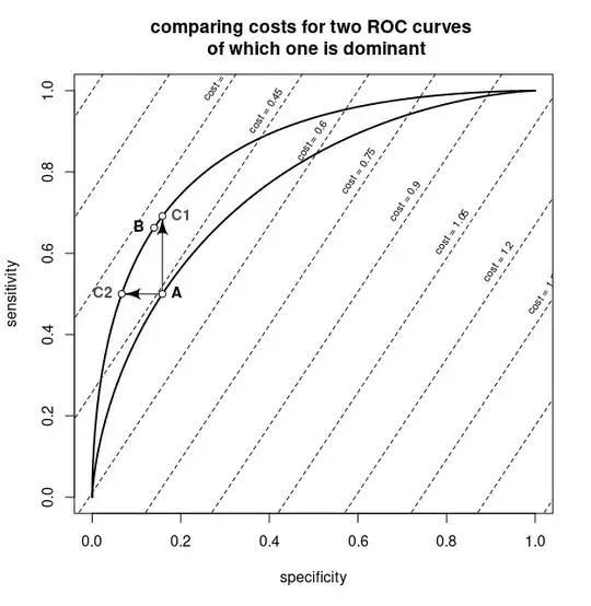
The plot shows the two ROC curves in thick lines. The diagonal lines are iso-curves for combinations of false positive rates and true positive rates with the same cost.
The point A is the optimal value for the non-dominant classifier. The arrows to points C1 and C2 show that the dominant classifier has two points that are as least as good (lower cost) than the optimal point for the non-dominant classifier. The point B is the optimum for the dominant classifier and is at least as good as the points C1 and C2. Since the cost in point B is equal or lower than the costs in points C1 and C2, and the costs in points C1 and C2 are lower than the cost in point A, the optimum of the dominant classifier has to be at equal or lower cost than the optimum for the non-dominant classifier.
In more complex situations, like considering noisy ROC curves, the situation might be different. For example, the dominant ROC curve might be dominant due to overfitting and lead to a bad choice of the threshold.
R-code for the plot:
xs = seq (-5,5, 0.01)
f = dnorm(1)/dnorm(0)
plot the two curves
plot(pnorm(xs,0.5),pnorm(xs,-0.5), type = "l", lwd = 2, xlab = "specificity", ylab = "sensitivity",
     main = "comparing costs for two ROC curves \n of which one is dominant")
lines(pnorm(xs,0.75),pnorm(xs,-0.75), lwd = 2)
plot the isolines
for (cost in seq(-1.65,1.65,0.15)) {
  lines(xs, 1-(cost-xs)/f, lty = 2)
  xt = 0.075+cost*0.7
  text(xt,1-(cost-xt)/f+0.05,paste0("cost = ",cost),srt=55, cex = 0.7)
}
the two arrows
shape::Arrows(pnorm(-0.5,0.5),pnorm(-0.5,-0.5), pnorm(-0.5,0.5), pnorm(qnorm(pnorm(-0.5,0.5),0.75),-0.75), arr.adj = 1, arr.type = "curved")
shape::Arrows(pnorm(-0.5,0.5),pnorm(-0.5,-0.5), pnorm(qnorm(pnorm(-0.5,-0.5),-0.75),0.75), pnorm(-0.5,-0.5), arr.adj = 1, arr.type = "curved")
points C1 and C2
points(pnorm(-0.5,0.5), pnorm(qnorm(pnorm(-0.5,0.5),0.75),-0.75), pch = 21, bg = 0)
points(pnorm(qnorm(pnorm(-0.5,-0.5),-0.75),0.75), pnorm(-0.5,-0.5), pch = 21, bg = 0)
text(pnorm(-0.5,0.5), pnorm(qnorm(pnorm(-0.5,0.5),0.75),-0.75), "C1", pos = 4, font = 2, col = rgb(0.3,0.3,0.3))
text(pnorm(qnorm(pnorm(-0.5,-0.5),-0.75),0.75), pnorm(-0.5,-0.5), "C2", pos = 2, font = 2, col = rgb(0.3,0.3,0.3))
points A and B
points(pnorm(-0.5,0.5),pnorm(-0.5,-0.5), pch = 21, bg = 0)
text(pnorm(-0.5,0.5),pnorm(-0.5,-0.5), "A", pos = 4, font = 2)
points(pnorm(-0.33,0.75),pnorm(-0.33,-0.75), pch = 21, bg = 0)
text(pnorm(-0.33,0.75),pnorm(-0.33,-0.75), "B", pos = 2, font = 2)
