It turns out we can obtain an exact analytical solution.
Because $(x_t, x_{t+1}, x_{t+2})$ has a (trivariate) Normal distribution (as will be proven below), any linear combination is Normal too, such as $(X,Y)=(x_{t+1}-x_t, x_{t+2}-x_t).$ Clearly this has zero expectation and so its distribution will be determined by its variance-covariance matrix,
$$\operatorname{Var}((X,Y)) = \Sigma_{X,Y} = \pmatrix{\operatorname{Var}(x_{t+1}-x_t) & \operatorname{Cov}(x_{t+1}-x_t,\ x_{t+2}-x_t)\\\operatorname{Cov}(x_{t+2}-x_t,\ x_{t+1}-x_t) & \operatorname{Var}(x_{t+2}-x_t)}.$$
Use the recursive definition of the series to work out these values, starting with
$$\begin{aligned}
x_{t+1} - x_t &= (b-1)x_t + u_{t+1};\\
x_{t+2}-x_t &= b\,x_{t+1}+u_{t+2} - x_t = b(b\,x_t + u_{t+1}) + u_{t+2} - x_t \\&= (b^2-1)x_t + b\,u_{t+1}+u_{t+2}.
\end{aligned}$$
Everything is in terms of linear combinations of the independent Normal variables $(x_t, u_{t+1}, u_{t+2}).$ This makes $(X,Y)$ multivariate Normal, as previously claimed. Let's turn to computing $\Sigma_{X,Y}.$
Presumably the series $(x_t)$ is stationary, which implies $\operatorname{Var}(x_t) = \sigma^2$ is the same for all $t.$ Thus
$$\sigma^2 = \operatorname{Var}(x_{t}) = \operatorname{Var}(bx_{t-1} + u_{t}) = b^2\sigma^2 + 1,$$
with the solution
$$\operatorname{Var}(x_{t}) = \sigma^2 = \frac{1}{1-b^2}.$$
The rest of the variance calculation now falls into place:
$$\operatorname{Var}(x_{t+1}-x_t) = \operatorname{Var}((b-1)x_t + u_{t+1}) = (b-1)^2\sigma^2 + 1 = \frac{2}{1+b}; $$
$$\operatorname{Var}(x_{t+2}-x_t) = \operatorname{Var}((b^2-1)x_t + bu_{t+1} + u_{t+2}) = (b^2-1)^2\sigma^2 + b^2 + 1 = 2$$
$$\operatorname{Cov}(x_{t+1}-x_t, x_{t+2}-x_t) = (b-1)(b^2-1)/\sigma^2 + b = 1.$$
That is, the variance-covariance matrix of $(X,Y)$ is simply
$$\Sigma_{X,Y} = \pmatrix{\frac{2}{1+b} & 1 \\ 1 & 2}.$$
Its correlation coefficient is therefore
$$\rho = \frac{1}{\sqrt{2/(1+b)\times 2}} = \frac{\sqrt{1+b}}{2}.$$
The solution method at https://stats.stackexchange.com/a/139090/919, to find the density of the maximum of two correlated Normal variables with equal variances, can directly be extended to an arbitrary bivariate Normal distribution with (say) mean $(\mu_x,\mu_y),$ positive standard deviations $(\sigma_x, \sigma_y),$ and correlation $\rho.$ Since nothing new is involved--this is merely a matter of changing the units of measurement of the two variables--I will just state the results.
The density of the maximum $Z=\max(X,Y)$ is given by the sum of two terms. The first one (where $X \ge Y$) contributes
$$\phi(z;\ \mu_x, \sigma_x)\ \Phi\left(z;\ h(z; \mu, \sigma, \rho),\ \sigma_y \sqrt{1-\rho^2}\right)$$
where $\phi$ is the Normal density (with given mean and standard deviation), $\Phi$ is the Normal distribution function (with the same parameter meanings), and
$$h(z; \mu, \sigma, \rho) = E[Y\mid X=z] = \mu_y + \frac{\sigma_y}{\sigma_x}\, \rho\, (z - \mu_x)$$
is the conditional expectation of the second variable given the first equals $z.$
The second term is obtained by switching the roles of the variables (so that $Y\ge X$): although $z$ (representing their maximum) remains the same in the formula and $\rho$ also is unchanged, $\mu$ and $\sigma$ are reversed.
Here, to be fully explicit, is an R implementation of the density function of $Z$ based directly on this description.
#
# Density of the maximum of a nondegenerate bivariate Normal.
#
dnorm2max <- function(z, mu=c(0,0), sigma=c(1,1), rho=0) {
  # The conditional expectation at `z`.
  h <- function(z, m, s) m[2] + s[2] / s[1] * rho * (z - m[1])
The contribution of one (infinitesimal) strip.
f <- function(z, m, s) dnorm(z, m[1], s[1]) *
                         pnorm(z, h(z, m, s), s[2] * sqrt(1 - rho^2))
Return the total from the vertical and horizontal strips.
f(z, mu, sigma) + f(z, rev(mu), rev(sigma))
}
As a check, this figure displays a histogram of $Z$ from a simulation of length 100,000, on which I have superimposed the graph of dnorm2max. The agreement is excellent.

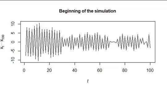
This specific example helps give some insight and helps inform our intuition. Because $b\approx -1,$ this is a strongly anticorrelated series: its values tend to oscillate between above-mean and below-mean numbers.
The variance of the first difference $x_{t+1}-x_t,$ equal to $50,$ is relatively large. The two-step difference $x_{t+2}-x_t$ only has a variance of $2,$ indicating that each first difference is very nearly reversed on the next step.
The correlation between these two variables--the one-step and two-step differences--is a low $0.1,$ however. Consequently, the maximum of the two differences is very likely to be the first one when it is positive, and otherwise it is likely to be the second one when the first is negative. The result therefore looks a little like an equal mixture of a Normal variable with variance $2$ (green in the next figure) and a half-Normal variable with variance $50$ (blue).

Finally, an attractive way to estimate the distribution of $Z$ (or any of its properties, such as percentiles) would be to estimate the parameter $b$ of the series $(x_t).$ (Realistically, you likely have to estimate $\sigma^2$ as well.) You can propagate the standard errors using the Delta method. When your estimates are based on optimizing a likelihood, this approach is rigorously justified.
With a sufficiently long realization of this time series model you could, of course, estimate the distribution of $Z$ from its empirical distribution. This is likely worthwhile doing as a check of your estimates.


