You can estimate Lambert W x Gaussian distributions and transformations using IGMM as follows (from your data.csv file).
yy <- read.csv("~/Downloads/data.csv")[, "x"]
library(LambertW)
test_normality(yy)

As you said, the data is clearly non-Gaussian with huge kurtosis (319) and negative skewness. Thus a natural candidate marginal model of your data is a double heavy-tailed Lambert W x Gaussian distribution (type = "hh"), which estimates heavy tails but with difference estimates for left and right tail.
mod <- IGMM(yy, "hh")
mod
 Parameter estimates:
 mu_x    sigma_x delta_l delta_r
 0.184   0.052   1.331   0.603
As expected from density and qqplot above, the left tail is much heavier than the right and not even first order moments exist ($\hat{\delta}_l > 1$). The back-transformed data can be obtained using
xx <- get_input(mod)
test_normality(xx)

and has kurtosis $3$, skewness $0.0$ as it was obtained via methods of moments (IGMM()). However, it's still clearly not Gaussian as it has a multi-modal distribution; especially a strong peak concentration / peak around the mean $\hat{\mu}_X = 0.184$. I took a close look at the original data around $\hat{\mu}_X = 0.184$ and found that this is actually occurring in the original data. It would be good to understand where these exact same values come from (some sort of default -- constant -- value in your measurements?):
yy.center <- yy[yy > mod$tau["mu_x"] - 0.05 & yy <  mod$tau["mu_x"] + 0.05]
test_normality(yy.center)
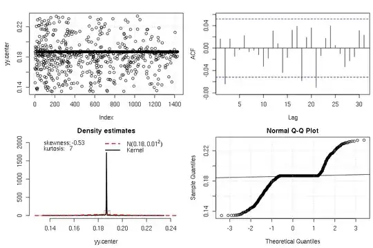
Also note that as we go from left to right the the density of x -- especially for values $x > \mu_X$ -- decreases, i.e., it seems like your 'x' variable depends on some other variable not included in your data (is this ordered by time?).
To summarize, we found that your data is
a. not only heavy-tailed but also (significantly) skewed,
b. non i.i.d., and
c. has more than one mode with some default constant values at $y \approx 0.184$.
All these findings are not visible in the original data, but only in the latent Gaussian transformed data. Depending on your problem and questions you aim to answer (see X-Y problem that Glen_b referenced) this might be useful information to have.
I do note that estimating this via MLE_LambertW(yy, distname="normal", type="hh")gives degenerate solutions. Not sure why this occurs, but my guess is because of the multi-modality (non-Normality) of the latent data, where the MLE has issues when assuming a unimodal Gaussian. Interesting question from a methodology pov.


