Joining spatial polygons by code in R?

Question

I am in the process of creating a spatial polygon map for the Valencia region in Spain. I asked the question in StackOverflow (https://stackoverflow.com/q/19791210/709777) and could produce the map.

Now I need to add an additional layer to the map. In my case I have a list of 30 areas with all city codes in the area. I would like to group all polygons in every area to overlay my map. I thought I could subset the 30 areas and then join polygons, maybe then create a shapefile with that 30 polygons to use in other R scripts.

The area-code list is in a different data frame than the polygons so I have to merge/join both of them.

What I'm trying is something similar to what is explained in https://gis.stackexchange.com/a/63696/9227. I just need to overlay a black line on the map showing the new 30 polygons.

Is it possible to group polygons based on a code list?

---

As suggested by @jbaums I've uploaded code and data.

First the R code I'm using to produce the maps:

require("rgdal")
require("maptools")
require("ggplot2")
require("plyr")
require("stringr")
library("mapproj")
library("gpclib")

gpclibPermit()

# Municipality and province limits
system("cp ../FILES/poligonos* ./",intern=T)

# read cities (just for plotting location of main cities)
main.cities=read.csv("ciutats.csv",header=F,sep=",",col.names=c("zona","codigoine","mean_lon","mean_lat","nombre"),colClasses=c("numeric","character","numeric","numeric","character"))

# read municipality polygons
esp     <- readOGR(dsn=".", layer="poligonos_municipio_etrs89")
muni    <- subset(esp, esp$PROVINCIA == "46" | esp$PROVINCIA == "12" | esp$PROVINCIA == "3")

# fortify and merge: muni.df is used in ggplot
muni@data$id <- rownames(muni@data)
muni.df <- fortify(muni)
muni.df <- join(muni.df, muni@data, by="id")

# read province polygons
prov = readOGR(dsn=".", layer="poligonos_provincia_etrs89")
pr=subset(prov, prov$CODINE == "46" | prov$CODINE == "12" | prov$CODINE == "03" )
pr@data$id = rownames(pr@data)
pr.points = fortify(pr, region="id")
pr.df = join(pr.points, pr@data, by="id")

# Maps for three days

for (k in 1:3) {

name.dat=paste("niveles-dia",k,".csv",sep="") # Level data are in files niveles-diaX.csv
fdat<-c(name.dat)                               

# read levels data
temp.data <- read.csv(fdat, header=F, sep=" ",col.names=c("codigo","nivel"), na.string="NA", dec=".", strip.white=TRUE)
temp.data$codigo <- str_pad(temp.data$codigo, width = 5, side = 'left', pad = '0')

# merge temperature and muni data
muni2.df <- merge(muni.df, temp.data, by.x="CODIGOINE", by.y="codigo", all.x=T, a..ly=F)

# merge temperature-muni data with cities data
muni3.df <- merge(muni2.df, main.cities, by.x="CODIGOINE", by.y="codigoine", all.x=T, a..ly=F)

# create the map layers
name.png=paste("CV-dia",k,".png",sep="") # Nom del fitxer per día
fpng<-c(name.png)

png(fpng, width = 1024, height = 768, units = 'px') # Start png output
ggp <- ggplot(data=muni2.df, aes(x=long, y=lat, group=group)) 
ggp <- ggp + geom_polygon(aes(fill=nivel))         # draw polygons
ggp <- ggp + geom_path(color="grey", linestyle=2)  # draw boundaries
ggp <- ggp + coord_equal() + xlab(" ") + ylab(" ")
ggp <- ggp + scale_fill_gradientn(colours=c("green","yellow","orange","red"),na.value = "transparent",
                     breaks=c(0,1,2,3),labels=c("Normal","Moderado","Alto","Extremo"),
                     limits=c(0,3))
ggp <- ggp + coord_map("lagrange")

# Adding main.cities layer
ggp1 <- ggp + geom_point(data=muni3.df, aes(x=mean_lon, y=mean_lat),size=2)
ggp1 <- ggp1 + geom_text(data=muni3.df, aes(x=mean_lon, y=mean_lat, label=nombre), hjust=0, family="Courier", fontface="italic", size=6)
ggp1 <- ggp1 + geom_path(data=pr.df, aes(x=long, y=lat, group=group),color="black", size=0.3)

# render the map
print(ggp1)
dev.off() # close plot and save to disk

remove('fdat','fpng','muni2.df','muni3.df')

}  # End of 3-day loop

Then the data files:

• ciutats.csv: https://www.dropbox.com/s/lycqdmo31zaeqtu/ciutats.csv?dl=0
• polygons (tar gzipped file): https://www.dropbox.com/s/r3kjrlfwxcm7ndb/poligons.tar.gz?dl=0
• niveles-dia1.csv (map levels): https://www.dropbox.com/s/alo7lr8x70d1ra4/niveles-dia1.csv?dl=0
• info-onades.csv (city and area codes): https://www.dropbox.com/s/38qp2r1czfbdzh1/info-onades.csv?dl=0

This is the map I am getting by now:

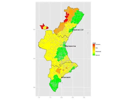
Now I would like to create 30 polygons/lines from data at info-onades.csv to overlay on this map.

---

Working code, with help from @jbaums

# Loading libraries
library("rgdal")
library("maptools")
library("ggplot2")
library("plyr")
library("stringr")
library("mapproj")
library("gpclib")
library("raster")
library("rgeos")

gpclibPermit()

# Read info on municipalities and area codes
info=read.csv("info-onades.csv",header=F,sep=",",col.names=c("zona","codigoine","mean_lon","mean_lat","nombre"),colClasses=c("numeric","character","numeric","numeric","character"))

# Subset municipal polygons to selected provinces (province codes 46, 12 and 3)
muni <- subset(readOGR('.', 'poligonos_municipio_etrs89', encoding='UTF-8'), PROVINCIA %in% c('46', '12', '3'))

# fortify and merge: muni.df is used later in ggplot
muni@data$id <- rownames(muni@data)
muni.df <- fortify(muni)
muni.df <- join(muni.df, muni@data, by="id")

# Create muni_area to aggregate municipalities in 30 areas (aggregate by column "zona")
# merge by codigoine to add zona column to muni.new and then aggregate by zona in muni_area
muni.new <- merge(muni, info, by.x='CODIGOINE', by.y='codigoine',all.x=TRUE, all.y=FALSE)
muni_area <- raster::aggregate(muni.new,'zona')

# Fortify and merge to create the data frame ggplot will overlay on the base map
muni_area@data$id <- rownames(muni_area@data)
muni_area.df <- fortify(muni_area)
muni_area.df <- join(muni_area.df, muni_area@data, by="id")

# read and fortify province
prov = readOGR(dsn=".", layer="poligonos_provincia_etrs89")
pr=subset(prov, prov$CODINE == "46" | prov$CODINE == "12" | prov$CODINE == "03" )
pr@data$id = rownames(pr@data)
pr.points = fortify(pr, region="id")
pr.df = join(pr.points, pr@data, by="id")

# Loop for plotting three maps

for (k in 1:3) {

  # Daily data file name
  name.dat=paste("niveles-dia",k,".csv",sep="")   
  fdat<-c(name.dat)                               

  # Read temperature level data
  temp.data <- read.csv(fdat, header=F, sep=" ",col.names=c("codigo","nivel"), na.string="NA", dec=".", strip.white=TRUE)
  temp.data$codigo <- str_pad(temp.data$codigo, width = 5, side = 'left', pad = '0')

  # merge temperature and muni data. muni2.df will be used by ggplot
  muni2.df <- merge(muni.df, temp.data, by.x="CODIGOINE", by.y="codigo", all.x=T, a..ly=F)

  # Daily map file output name
  name.png=paste("CV-map-",k,".png",sep="") # Nom del fitxer per día
  fpng<-c(name.png)

  png(fpng, width = 1024, height = 768, units = 'px') # Start png output

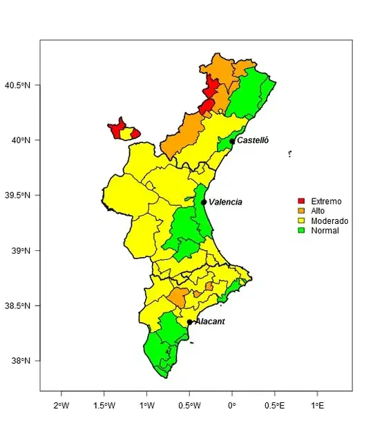
  # Mapping municipalities by level (nivel)
  ggp <- ggplot(data=muni2.df, aes(x=long, y=lat, group=group)) 
  ggp <- ggp + geom_polygon(aes(fill=nivel))         # draw polygons
  ggp <- ggp + geom_path(color="grey", linestyle=2)  # draw boundaries
  ggp <- ggp + coord_equal() + xlab(" ") + ylab(" ")
  ggp <- ggp + scale_fill_gradientn(colours=c("green","yellow","orange","red"),na.value = "transparent",
                                    breaks=c(0,1,2,3),labels=c("Normal","Moderado","Alto","Extremo"),
                                    limits=c(0,3))
  ggp <- ggp + coord_map("lagrange")

  # Overlay 30 areas
  ggp <- ggp + geom_path(data=muni_area.df, aes(x=long, y=lat, group=group),color="blue", size=0.3)
  # Overlay provinces
  ggp <- ggp + geom_path(data=pr.df, aes(x=long, y=lat, group=group),color="black", size=0.5)

  # Render the map
  print(ggp)
  dev.off() # close plot and save to disk

  remove('fdat','fpng','muni2.df') # clear variables for each map

}

And the final map (removed names of main cities in the prior map)

Answer 1

The short answer is that you can aggregate SpatialPolygons by one or more fields with raster::aggregate.

The long answer is that this is how I'd approach your entire problem with either base plotting, or lattice:

1. Data preparation:

   library(rgdal)
   library(raster)
   
   # Read in data on major cities
   cities <- read.csv("ciutats.csv", header=FALSE, encoding='UTF-8',
                      col.names=c('zona', 'codigoine', 'mean_lon', 'mean_lat', 'nombre'))
   
   # Read in province polygons
   pr <- subset(readOGR('.', 'poligonos_provincia_etrs89', encoding='UTF-8'),
                CODINE %in% c('46', '12', '03'))
   
   # Subset municipal polygons to selected provinces
   muni <- subset(readOGR('.', 'poligonos_municipio_etrs89', encoding='UTF-8'),
                  PROVINCIA %in% c('46', '12', '3'))
   
   # Read in city codes, pad zeroes and coerce nivel to factor for plotting cnvenience
   codigo_nivel <- read.table('niveles-dia1.csv', col.names=c('codigo', 'nivel'), 
                              stringsAsFactors=FALSE)
   codigo_nivel$codigo <- sprintf('%05d', codigo_nivel$codigo)
   codigo_nivel$nivel <- factor(codigo_nivel$nivel, 
                            labels=c('Normal', 'Moderado', 'Alto', 'Extremo'))
   
   # Add codigo and nivel to muni
   muni <- merge(muni, codigo_nivel, by.x="CODIGOINE", by.y="codigo",
                 all.x=TRUE, all.y=FALSE)
   
   # Read in area data and correct mismatching names
   info <- read.csv('info-onades.csv', header=FALSE, encoding='UTF-8',
                    col.names=c('area', 'codigo', 'lon', 'lat', 'nombre'),
                    stringsAsFactors=FALSE)
   info$nombre[which(info$nombre == 'Alacant/Alicante')] <- 'Alacant/Alicante'
   info$nombre[which(info$nombre == 'Xert')] <- 'Chert/Xert'
   
   # Add area info to muni
   muni <- merge(muni, info[, c('area', 'nombre')], by.x='NOMBRE', by.y='nombre', 
                 all.x=TRUE, all.y=FALSE)
   
   # Aggregate muni by area
   muni_area <- raster::aggregate(muni, 'area')
   

2. Let's plot:

   # Define colour scheme
   colr <- c('green', 'yellow', 'orange', 'red')
   
   # Plotting with base R
   plot(muni, border=NA, col=colr[as.numeric(muni$nivel)], axes=TRUE, las=1)
   plot(muni_area, add=TRUE)
   plot(pr, add=TRUE, lwd=2)
   points(cities$mean_lon, cities$mean_lat, pch=20, cex=2)
   text(cities$mean_lon, cities$mean_lat, cities$nombre, font=4, pos=4)
   legend('right', c('Extremo', 'Alto', 'Moderado', 'Normal'), fill=rev(colr), bty='n')
   

   

   # Plotting with lattice and latticeExtra
   library(latticeExtra)
   spplot(muni, 'nivel', col=NA, col.regions=colr, scales=list(draw=TRUE, tck=c(1, 0)),
          xlim=bbox(muni)[1, ] + c(-0.25, 0.25), # otherwise plot is a bit cramped
          ylim=bbox(muni)[2, ] + c(-0.25, 0.25)) + 
     layer(sp.polygons(muni_area)) +
     layer(sp.polygons(pr, lwd=2)) +
     layer(lpoints(cities$mean_lon, cities$mean_lat, pch=20, cex=2, col=1)) +
     layer(ltext(cities$mean_lon, cities$mean_lat, cities$nombre, pch=20, font=4, pos=4))
   

   

Note that above I've suppressed plotting of the muni polygon borders for small municipal entities. Change col=NA as desired to plot these.