How to display all trigonometric function plots in a table?

Question

For my maths summary I am trying to make a table with all function plots of the trigonometric functions (Something like the picture below, but including the inverses). Since my space is limited to 12 pages I want some of them to be vertically aligned to save some space, just like in the picture. I am fairly new to Latex and I tried doing this using tabular. However the plots are bit too far on the right - I want them perfectly centered. How can I do this?

My other problem is that if I try to plot functions like tan, csc, sec, arcsin,arccos,... they either produce an error or mess everything up. How can I plot these functions?

I also couldn't find any templates with all the trig functions summarized, which I found odd since I thought that would be something I am not the first person in need of. Is there a secret place where such files are shared?

Here is my code for three functions (I included cosine twice so I have something to display):

\documentclass{article}
\usepackage[utf8]{inputenc}
\title{testtt}
\usepackage{amsmath}    \usepackage{amsfonts}   \usepackage{amssymb}
\usepackage{amsthm}     \usepackage{latexsym}   \usepackage{mathtools}
\usepackage{tikz}
\begin{document}
\newcommand{\xMin}{-9}
\newcommand{\xMax}{9}
\newcommand{\yMin}{-3}
\newcommand{\yMax}{3}
\begin{tabular}{ c c }
\begin{tikzpicture}[>=stealth,scale=0.4]
    \draw[very thin,color=gray,scale={pi/2}] ({\xMin((1)/(2))+0.01},-6/pi+0.01) grid ({\xMax(1/2)-0.01},7/pi-0.01);
    \draw node at ({pi},0) [below] {${\pi}$};
    \draw node at ({2pi},0) [below] [xshift=1pt] {${2\pi}$};
    \draw node at ({-pi},0) [below] [xshift=-2pt]  {${-\pi}$};
    \draw node at ({-2pi},0) [below] [xshift=-2pt] {${-2\pi}$};
\draw node at (0,1) [left] {$1$};
\draw node at (0,2) [left] {$2$};
\draw node at (0,-1) [left] {$-1$};
\draw node at (0,-2) [left] {$-2$};


\draw [-&gt;] [thick] ({\xMin*(pi/4)},0) -- ({\xMax*(pi/4)+0.5},0) 
    node [right] {$x$};
\draw [-&gt;] [thick] (0,-3) -- (0,3.5)
    node [above] {$y$};

\draw [-,thin,black,domain={-2*pi}:{2*pi},samples=100] 
plot (\x, {sin(\x*180/pi)}) node[above] {$f(x) = \sin(x)$};


\end{tikzpicture} &
\begin{tikzpicture}[>=stealth,scale=0.4]
    \draw[very thin,color=gray,scale={pi/2}] ({\xMin((1)/(2))+0.01},-6/pi+0.01) grid ({\xMax(1/2)-0.01},7/pi-0.01);
    \draw node at ({pi},0) [below] {${\pi}$};
    \draw node at ({2pi},0) [below] [xshift=1pt] {${2\pi}$};
    \draw node at ({-pi},0) [below] [xshift=-2pt]  {${-\pi}$};
    \draw node at ({-2pi},0) [below] [xshift=-2pt] {${-2\pi}$};
\draw node at (0,1) [left] {$1$};
\draw node at (0,2) [left] {$2$};
\draw node at (0,-1) [left] {$-1$};
\draw node at (0,-2) [left] {$-2$};


\draw [-&gt;] [thick] ({\xMin*(pi/4)},0) -- ({\xMax*(pi/4)+0.5},0) 
    node [right] {$x$};
\draw [-&gt;] [thick] (0,-3) -- (0,3.5)
    node [above] {$y$};

\draw [-,thin,black,domain={-2*pi}:{2*pi},samples=100] 
plot (\x, {cos(\x*180/pi)}) node[above] {$f(x) = \cos(x)$};


\end{tikzpicture} \
\begin{tikzpicture}[>=stealth,scale=0.4]
    \draw[very thin,color=gray,scale={pi/2}] ({\xMin((1)/(2))+0.01},-6/pi+0.01) grid ({\xMax(1/2)-0.01},7/pi-0.01);
    \draw node at ({pi},0) [below] {${\pi}$};
    \draw node at ({2pi},0) [below] [xshift=1pt] {${2\pi}$};
    \draw node at ({-pi},0) [below] [xshift=-2pt]  {${-\pi}$};
    \draw node at ({-2pi},0) [below] [xshift=-2pt] {${-2\pi}$};
\draw node at (0,1) [left] {$1$};
\draw node at (0,2) [left] {$2$};
\draw node at (0,-1) [left] {$-1$};
\draw node at (0,-2) [left] {$-2$};


\draw [-&gt;] [thick] ({\xMin*(pi/4)},0) -- ({\xMax*(pi/4)+0.5},0) 
    node [right] {$x$};
\draw [-&gt;] [thick] (0,-3) -- (0,3.5)
    node [above] {$y$};

\draw [-,thin,black,domain={-2*pi}:{2*pi},samples=100] 
plot (\x, {cos(\x*180/pi)}) node[above] {$f(x) = \cos(x)$};


\end{tikzpicture}
\end{tabular}
\end{document}

this

Your plots appear "are bit too far on the right" since the table containing them is wider than the textwidth. (You should receive an overfull box warning). To overcome this, you could for example decrease the margins using the geometry packge. — leandriis, Jan 09 '21 at 11:48

cmhughes · Accepted Answer · 2021-01-10T15:13:13.230

I would advocate using the pgfplots package for this type of graphic.

It allows you to use the following, for example

  \begin{tikzpicture}
    \begin{axis}
      \addplot[timtam]expression[domain=-3.5:3.5]{sin(x)};
    \end{axis}
  \end{tikzpicture}

Here's a couple of demonstrations; adjust as you see fit. For reference, see also Axis with trigonometric labels in PGFPlots, for example.

option 1 : using minipages, and individual plots

% arara: pdflatex
\documentclass{article}
\usepackage{geometry}
\usepackage{pgfplots}
\pgfplotsset{
  % framing the graphs
  framed/.style={
      axis background/.style ={draw=blue,fill=yellow!20,rounded corners=3ex}},
  % line style
  timtam/.style={
      color=red,mark=none,line width=1pt},
  % every axis
  every axis/.append style={
      axis x line=middle,    % put the x axis in the middle
      axis y line=middle,    % put the y axis in the middle
      axis line style={->},  % arrows on the axis
      xlabel={$x$},          % default put x on x-axis
      ylabel={$y$},          % default put y on y-axis
      scale only axis,       % otherwise width won't be as intended: http://tex.stackexchange.com/questions/36297/pgfplots-how-can-i-scale-to-text-width
      xtick={-3.14159265359,-1.57079632679,1.57079632679,3.14159265359},
      xticklabels={$-\pi$,$-\pi/2$,$\pi/2$,$\pi$},
      xmin=-3.5, xmax=3.5,
      ymin=-2.3, ymax=2.3,
      trig format=rad,       % use radians
      framed,
      grid=both,
      width=\textwidth,
    },
  % not needed in the below, but you might like them for future
  asymptote/.style={
      color=red,mark=none,line width=1pt,dashed},
  soldot/.style={
      color=red,only marks,mark=*},
  holdot/.style={
      color=red,fill=white,only marks,mark=*},
}
% arrow style
\tikzset{>=stealth}
\begin{document}
\begin{minipage}{.33\textwidth}
  \begin{tikzpicture}
    \begin{axis}
      \addplot[timtam]expression[domain=-3.5:3.5]{sin(x)};
    \end{axis}
  \end{tikzpicture}
\end{minipage}
\begin{minipage}{.33\textwidth}
  \begin{tikzpicture}
    \begin{axis}
      \addplot[timtam]expression[domain=-3.5:3.5]{cos(x)};
    \end{axis}
  \end{tikzpicture}
\end{minipage}
\begin{minipage}{.33\textwidth}
  \begin{tikzpicture}
    \begin{axis}
      \addplot[timtam]expression[domain=-4.5:-1.58]{tan(x)};
      \addplot[timtam]expression[domain=-1.56:1.55]{tan(x)};
      \addplot[timtam]expression[domain=1.58:4.5]{tan(x)};
    \end{axis}
  \end{tikzpicture}
\end{minipage}%
\vspace{1cm}
\begin{minipage}{.33\textwidth}
  \begin{tikzpicture}
    \begin{axis}
      \addplot[timtam]expression[domain=-3.5:-3.2]{1/sin(x)};
      \addplot[timtam]expression[domain=-3.1:-0.1]{1/sin(x)};
      \addplot[timtam]expression[domain=0.1:3.1]{1/sin(x)};
      \addplot[timtam]expression[domain=3.2:4.5]{1/sin(x)};
    \end{axis}
  \end{tikzpicture}
\end{minipage}
\begin{minipage}{.33\textwidth}
  \begin{tikzpicture}
    \begin{axis}
      \addplot[timtam]expression[domain=-4.5:-1.58]{1/cos(x)};
      \addplot[timtam]expression[domain=-1.56:1.56]{1/cos(x)};
      \addplot[timtam]expression[domain=1.58:4.5]{1/cos(x)};
    \end{axis}
  \end{tikzpicture}
\end{minipage}
\begin{minipage}{.33\textwidth}
  \begin{tikzpicture}
    \begin{axis}
      \addplot[timtam]expression[domain=-3.5:-3.2]{cot(x)};
      \addplot[timtam]expression[domain=-3.1:-0.1]{cot(x)};
      \addplot[timtam]expression[domain=0.1:3.1]{cot(x)};
      \addplot[timtam]expression[domain=3.2:4.5]{cot(x)};
    \end{axis}
  \end{tikzpicture}
\end{minipage}%
\end{document}

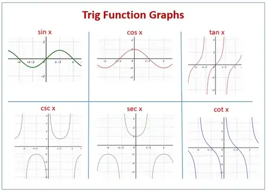
option 2: just like option 1, but with titles

If you'd like to add titles, we can use the following, for example; you'll see that the new part to the above is

      title style={at={(axis cs:0,-3.2)}}, %<------  NEW BIT

and then, within the code, I've used \begin{axis}[title={$y=\sin(x)$}].

% arara: pdflatex
\documentclass{article}
\usepackage{geometry}
\usepackage{pgfplots}
\pgfplotsset{
  % framing the graphs
  framed/.style={
      axis background/.style ={draw=blue,fill=yellow!20,rounded corners=3ex}},
  % line style
  timtam/.style={
      color=red,mark=none,line width=1pt},
  % every axis
  every axis/.append style={
      axis x line=middle,    % put the x axis in the middle
      axis y line=middle,    % put the y axis in the middle
      axis line style={->},  % arrows on the axis
      xlabel={$x$},          % default put x on x-axis
      ylabel={$y$},          % default put y on y-axis
      scale only axis,       % otherwise width won't be as intended: http://tex.stackexchange.com/questions/36297/pgfplots-how-can-i-scale-to-text-width
      xtick={-3.14159265359,-1.57079632679,1.57079632679,3.14159265359},
      xticklabels={$-\pi$,$-\pi/2$,$\pi/2$,$\pi$},
      xmin=-3.5, xmax=3.5,
      ymin=-2.3, ymax=2.3,
      trig format=rad,       % use radians
      framed,
      grid=both,
      width=\textwidth,
      title style={at={(axis cs:0,-3.2)}}, %<------  NEW BIT
    },
  % not needed in the below, but you might like them for future
  asymptote/.style={
      color=red,mark=none,line width=1pt,dashed},
  soldot/.style={
      color=red,only marks,mark=*},
  holdot/.style={
      color=red,fill=white,only marks,mark=*},
}
% arrow style
\tikzset{>=stealth}
\begin{document}
\begin{minipage}{.33\textwidth}
  \begin{tikzpicture}
    \begin{axis}[title={$y=\sin(x)$}]
      \addplot[timtam]expression[domain=-3.5:3.5]{sin(x)};
    \end{axis}
  \end{tikzpicture}
\end{minipage}
\begin{minipage}{.33\textwidth}
  \begin{tikzpicture}
    \begin{axis}[title={$y=\cos(x)$}]
      \addplot[timtam]expression[domain=-3.5:3.5]{cos(x)};
    \end{axis}
  \end{tikzpicture}
\end{minipage}
\begin{minipage}{.33\textwidth}
  \begin{tikzpicture}
    \begin{axis}[title={$y=\tan(x)$}]
      \addplot[timtam]expression[domain=-4.5:-1.58]{tan(x)};
      \addplot[timtam]expression[domain=-1.56:1.55]{tan(x)};
      \addplot[timtam]expression[domain=1.58:4.5]{tan(x)};
    \end{axis}
  \end{tikzpicture}
\end{minipage}%
\vspace{1cm}
\begin{minipage}{.33\textwidth}
  \begin{tikzpicture}
    \begin{axis}[title={$y=\csc(x)$}]
      \addplot[timtam]expression[domain=-3.5:-3.2]{1/sin(x)};
      \addplot[timtam]expression[domain=-3.1:-0.1]{1/sin(x)};
      \addplot[timtam]expression[domain=0.1:3.1]{1/sin(x)};
      \addplot[timtam]expression[domain=3.2:4.5]{1/sin(x)};
    \end{axis}
  \end{tikzpicture}
\end{minipage}
\begin{minipage}{.33\textwidth}
  \begin{tikzpicture}
    \begin{axis}[title={$y=\sec(x)$}]
      \addplot[timtam]expression[domain=-4.5:-1.58]{1/cos(x)};
      \addplot[timtam]expression[domain=-1.56:1.56]{1/cos(x)};
      \addplot[timtam]expression[domain=1.58:4.5]{1/cos(x)};
    \end{axis}
  \end{tikzpicture}
\end{minipage}
\begin{minipage}{.33\textwidth}
  \begin{tikzpicture}
    \begin{axis}[title={$y=\cot(x)$}]
      \addplot[timtam]expression[domain=-3.5:-3.2]{cot(x)};
      \addplot[timtam]expression[domain=-3.1:-0.1]{cot(x)};
      \addplot[timtam]expression[domain=0.1:3.1]{cot(x)};
      \addplot[timtam]expression[domain=3.2:4.5]{cot(x)};
    \end{axis}
  \end{tikzpicture}
\end{minipage}%
\end{document}

option 3: using groupplot

The output is as in option 2, but the input is, perhaps, more pleasing; note that this requires the groupplots library, annotated in the code below.

% arara: pdflatex
\documentclass{article}
\usepackage{geometry}
\usepackage{pgfplots}
\usepgfplotslibrary{groupplots}  %<------------ NEW BIT
\pgfplotsset{
  % framing the graphs
  framed/.style={
      axis background/.style ={draw=blue,fill=yellow!20,rounded corners=3ex}},
  % line style
  timtam/.style={
      color=red,mark=none,line width=1pt},
  % every axis
  every axis/.append style={
      axis x line=middle,    % put the x axis in the middle
      axis y line=middle,    % put the y axis in the middle
      axis line style={->},  % arrows on the axis
      xlabel={$x$},          % default put x on x-axis
      ylabel={$y$},          % default put y on y-axis
      scale only axis,       % otherwise width won't be as intended: http://tex.stackexchange.com/questions/36297/pgfplots-how-can-i-scale-to-text-width
      xtick={-3.14159265359,-1.57079632679,1.57079632679,3.14159265359},
      xticklabels={$-\pi$,$-\pi/2$,$\pi/2$,$\pi$},
      xmin=-3.5, xmax=3.5,
      ymin=-2.3, ymax=2.3,
      trig format=rad,       % use radians
      framed,
      grid=both,
      width=\textwidth,
      title style={at={(axis cs:0,-3.2)}},
    },
  % not needed in the below, but you might like them for future
  asymptote/.style={
      color=red,mark=none,line width=1pt,dashed},
  soldot/.style={
      color=red,only marks,mark=*},
  holdot/.style={
      color=red,fill=white,only marks,mark=*},
}
% arrow style
\tikzset{>=stealth}
\begin{document}
\begin{tikzpicture}
  \begin{groupplot}[
      group style={
          group name=my plots,
          group size=3 by 2,
        },
      width=.33\textwidth,
    ]
    \nextgroupplot[title={$y=\sin(x)$}]
      \addplot[timtam]expression[domain=-3.5:3.5]{sin(x)};
    \nextgroupplot[title={$y=\cos(x)$}]
      \addplot[timtam]expression[domain=-3.5:3.5]{cos(x)};
    \nextgroupplot[title={$y=\tan(x)$}]
      \addplot[timtam]expression[domain=-4.5:-1.58]{tan(x)};
      \addplot[timtam]expression[domain=-1.56:1.55]{tan(x)};
      \addplot[timtam]expression[domain=1.58:4.5]{tan(x)};
    \nextgroupplot[title={$y=\csc(x)$}]
      \addplot[timtam]expression[domain=-3.5:-3.2]{1/sin(x)};
      \addplot[timtam]expression[domain=-3.1:-0.1]{1/sin(x)};
      \addplot[timtam]expression[domain=0.1:3.1]{1/sin(x)};
      \addplot[timtam]expression[domain=3.2:4.5]{1/sin(x)};
    \nextgroupplot[title={$y=\sec(x)$}]
      \addplot[timtam]expression[domain=-4.5:-1.58]{1/cos(x)};
      \addplot[timtam]expression[domain=-1.56:1.56]{1/cos(x)};
      \addplot[timtam]expression[domain=1.58:4.5]{1/cos(x)};
    \nextgroupplot[title={$y=\cot(x)$}]
      \addplot[timtam]expression[domain=-3.5:-3.2]{cot(x)};
      \addplot[timtam]expression[domain=-3.1:-0.1]{cot(x)};
      \addplot[timtam]expression[domain=0.1:3.1]{cot(x)};
      \addplot[timtam]expression[domain=3.2:4.5]{cot(x)};
  \end{groupplot}
\end{tikzpicture}
\end{document}

If you need to number/reference the figures, then I'd recommend using the \caption command, perhaps employing the subfigure package.

This is exactly what I needed, thanks so much! Is there an easy way to add a label below the minipages? — timtam, Jan 09 '21 at 14:13
@timtam great, glad it worked :) I've updated with an option detailing the labels below the plots. — cmhughes, Jan 09 '21 at 16:12
@cmhughes nice! :) Just a question for my culture. Why not use group plot and prefer minipages? — JeT, Jan 09 '21 at 23:32
@jet no particular reason :) I have the minipage syntax to my fingertips, but haven't used group plots all that much — cmhughes, Jan 10 '21 at 08:12
@JeT thanks for this; I've added a demonstration using the groupplots library. The input is, to my mind, more pleasing :) thanks for highlighting it — cmhughes, Jan 10 '21 at 15:13

How to display all trigonometric function plots in a table?

1 Answers1

option 1 : using minipages, and individual plots

option 2: just like option 1, but with titles

option 3: using groupplot