How to define an interval on a Beta distribution pdf?

Question

I have a Beta distribution curve and need to complete the code to define and highlight a region on the curve as shown in the figure.

\documentclass[border=5pt]{standalone}
\usepackage{pgfplots}
\newcommand*\GnuplotDefs{
    Binv(p,q)=exp(lgamma(p+q)-lgamma(p)-lgamma(q));
    beta(x,p,q)=p<=0||q<=0?1/0:x<0||x>1?0.0:Binv(p,q)*x**(p-1.0)*(1.0-x)**(q-1.0);
}
\begin{document}
\begin{tikzpicture}
    \pgfmathsetmacro{\xmin}{0}
    \pgfmathsetmacro{\xmax}{1}
\begin{axis}[
    xmin=\xmin,
    xmax=\xmax,
    no markers,
]
    \addplot gnuplot [raw gnuplot] {
        \GnuplotDefs
        plot [x=\xmin:\xmax] beta(x,7,5);
    };
\end{axis}
\end{tikzpicture}
\end{document}

Answer 1

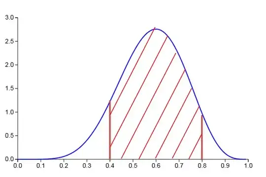
As John Kormylo already mentioned in the comment below the question filling the area between (parts) of curves can be done with the help of the fillbetween library of PGFPlots. For more details on how it works, please have a look at the comments in the code.

% used PGFPlots v1.14
% (code modified from <https://tex.stackexchange.com/a/368152/95441>)
\documentclass[border=5pt]{standalone}
\usepackage{pgfplots}
    % load the `fillbetween' library to fill (parts) of the area under a curve
    \usetikzlibrary{
        pgfplots.fillbetween,
    }
    \pgfplotsset{
        % use this `compat' level or higher so there is no need to prepend
        % every TikZ coordinate with `axis cs:'
        compat=1.11,
    }
    % define a command which stores all commands that are needed for every
    % `raw gnuplot' call
    \newcommand*\GnuplotDefs{
        % set number of samples
        set samples 51;
        %
        % define beta distribution function
        % (copied from <http://gnuplot.sourceforge.net/demo/prob.5.gnu>)
        Binv(p,q)=exp(lgamma(p+q)-lgamma(p)-lgamma(q));
        beta(x,p,q)=p<=0||q<=0?1/0:x<0||x>1?0.0:Binv(p,q)*x**(p-1.0)*(1.0-x)**(q-1.0);
    }
\begin{document}
\begin{tikzpicture}
        % define macros which are needed for the axis limits as well as for
        % setting the domain of calculation
        \pgfmathsetmacro{\xmin}{0}
        \pgfmathsetmacro{\xmax}{1}
    \begin{axis}[
        xmin=\xmin,
        xmax=\xmax,
        ymin=0,
        no markers,
        % to make the plot look nicer
        smooth,
    ]
        % (invisible) path at y = 0 which is later used for `fill between'
        \path [name path=origin]
            (\pgfkeysvalueof{/pgfplots/xmin},0) --
            (\pgfkeysvalueof{/pgfplots/xmax},0);

        % draw the Beta function
        \addplot+ [
            name path=Beta,
            thick,
        ] gnuplot [raw gnuplot] {
            % first call all the "common" definitions
            \GnuplotDefs
            % and then create the data tables
            % in GnuPlot `x` key is identical to PGFPlots `domain` key
            %
            % "plot" beta function
            plot [x=\xmin:\xmax] beta(x,7,5);
        };

        % fill the area under the Beta function in the given interval
            % define the boundaries of the interval
            \pgfmathsetmacro{\Lower}{0.4}
            \pgfmathsetmacro{\Upper}{0.8}
        \addplot [
            orange,
        ] fill between [
            of=origin and Beta,
            soft clip={domain=\Lower:\Upper},
        ];

        % because there is no real intersection between the two given
        % `name path's, we cannot use the `intersection segments' feature of
        % the fill between library, that is, why we invisibly draw the Beta
        % function again, but this time only using two samples at the start
        % and end of the interval ...
        \addplot+ [
            draw=none,
        ] gnuplot [raw gnuplot] {
            \GnuplotDefs
            set samples 2;
            %
            plot [x=\Lower:\Upper] beta(x,7,5);
        }
            % ... and add coordinates to the two points.
            coordinate [at start] (lower boundary)
            coordinate [at end]   (upper boundary)
        ;
        % These coordinates can now be used to draw the vertical lines
        \draw [red,very thick]
            (lower boundary) -- (lower boundary |- 0,0)
            (upper boundary) -- (upper boundary |- 0,0)
        ;
    \end{axis}
\end{tikzpicture}
\end{document}