Changepoints in R

Question

I have the following dataset:

results <- data.frame(Date = c("A", "B", "C", "D", "E", "F", "G", "H","I", "J", "K", "L", "M", "N", "O", "P", "Q", "R", "S"),
                  P1 = c(0.43, 0.45, 0.57, 0.15, 0.5, 0.33, 0.26, 0.81, 0.43, 0.48, 0.14, 0.26,-0.21, 0.27, 0.37, 0.33, 0.68, 0.15, 0.44))

I want to know, if there are statistically significant changes of my observations.

So I thought to use changepoint analysis.

First I used the bcp-Package, with the following code:

c <- bcp(results$P1)
plot(c) 

However, there are no changepoints according to this plot.

Then I used the "changepoint" package and the following code:

var=cpt.var(results$P1, method="PELT")
plot(var)

Here I get three possible changepoints, but not were I supposed them to be (for example not in M, but in N).

Can anybody explain me why? Or is there another way to show, if the values changed significantly from one observation to another?

Answer 1

IrishStat is correct in that you are trying to identify a change in mean, not a change in variance. Thus in the changepoint package you should be using mean=cpt.mean(results$P1, method="PELT") instead. As for the bcp package this gives no changes in mean.

The cpt.var function gave 3 changes in variance because the variances of each part, calculated using

segvar=param.est(var)$variance
segvar
>0.02126190 0.09944762 0.00080000 0.07043333

segvar[-1]/segvar[-length(segvar)]
>4.677267637  0.008044436 88.041666667

Typically changes in variance are detected with roughly 80% power or more if the ratio of neighbouring variances is greater than 3 (or less than 1/3). The ratio of these variances clearly fits this paradigm which is why the changes were detected but not necessarily in the places you would have expected to identify a change in mean.

Note that this is all based on a penalty that only penalizes the number of changepoints. This is why segment lengths of 2/3 observations are detected. If the application suggests segments of small lengths such as these are implausible then I would use a penalty that penalizes segment length too (or set a minimum segment length).

See introductory references at www.changepoint.info for more background details on changepoint analysis. There is also a list of various changepoint open source software packages there.

Answer 2

Change Point analysis can mean detecting parameter changes OR changes in error variance OR changes in the Expected Value. Your example is simply the latter. Detecting change points in the Expected Value is called Intervention Detection http://www.unc.edu/~jbhill/tsay.pdf . This has been significantly enhanced in a product called http://www.autobox.com/cms/ which I helped develop that even incorporates user-specified predict series. I took your 19 values and AUTOBOX detected change points at M,H, and Q (13th,8th and 17th values) Note well that in general ARIMA structure has to be taken into account in time series analysis. In this case there is no provable arima structure ( autoregressive memory). It appears to me that your free software has a cost.

Exploratory Data Analysis as championed by Tukey, Box et.al. speaks to extracting hypothesis/information from the actual data such as the form of the ARIMA model, the detection of anomalies , changes in parameters etc. all of which do not require specific quantitative hypothesis promulgated before the data arrives. If one is lucky enough to have these hypothesis handy one can of course test them. Modern analytics actually learn from the data. What you knew (visually or scientifically) to be unusual was indeed detectable. I would say that the Tsay reference is an example of a trustworthy procedure.

Answer 3

For this 19-values series, some inconsistency exists among the methods--as expected when it comes to statistics (e.g., "no" changes detected by bcp, no breakpoint by the CUSUM and Quandt likelihood ratio tests in strucchange, no change in mean by changepoint, and three pulse-like changes by autobox). Let me give my two cents and throw some biased interpretations, which could be very wrong. Overall, I think that the different results are not directly comparable for reasons like differences in assumptions, model spaces assumed, and test statistics involved.

PURELY from an information-theoretic point of view, here is the ranking of several alternative models (no autocorrelation assumed) in terms of BIC (the smaller, the better):

M1. bic =-12.42 for the 3-pluses model by autbox (pluses at 8th,13th,& 17th)
M2. bic = -9.10 for a 2-pluses model with changes at 8th and 13th points
M3. bic = 1.601 for a mean-shift model at the 11-th point
M4. bic = 1.837 for a mean model without any changepoint

So, in terms of delta_BIC, the evidence favoring the AUTOBOX model (M1) over the no-change model (M4) is very strong. If we limit ourselves only to be the space of mean-shift models, the best model (again in terms of BIC) appears to the one-changepoint model M3 rather than the no-change model M4, although the evidence favoring M3 over M4 is rather weak. Again, this is purely interpreted in one information-theoretic criterion; the results for sure will be different if switching to classical tests.

Jumping into the Bayesian world, I interpret the bcp result a little bit differently from others. Below is the bcp result. On the first look, there is no salient peak in the probability curve, but if plotted in the finer scale, there are some small peaks and also the fitted curve differs from the a flat line, apparently due to the model averaging nature of the bayesian method. More specifically, according to the bcp output, on average the number of changepoints is 0.98, close to 1. So, my interpretation is that bcp indeed suggests an overall change in mean, but there is no strong model evidence to pinpoint an exact location so that the probability curve is spread out.

Here are also some extra results from another Bayesian changepoint detection package Rbeast my team developed (available in R, Python, and Matlab). Below is the result with a full Bayesian model, giving an average of 0.56 changepoints.

Next is the result with an empirical Bayesian model based on BIC

library(Rbeast)
y = c(0.43, 0.45, 0.57, 0.15, 0.5, 0.33, 0.26, 0.81, 0.43, 0.48, 0.14, 0.26,-0.21, 0.27, 0.37, 0.33, 0.68, 0.15, 0.44)
o = beast(y, season='none', method='bic')
plot(o)
barplot(names.arg=0:3, o$trend$ncpPr)

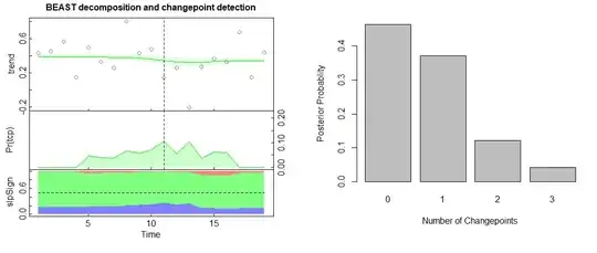
On average, there is 0.746 changepoint, with the most likely location being #11th (the dashed line in the figure below), which corresponds to the best one-changepoint model M3 obtained by optimizing BIC.

To mimic autobox, this is the result by allowing spike-like outliers without any mean changepoint allowed (i.e., tcp.minmax=c(0,0)).

o = beast(y, season='none', tcp.minmax=c(0,0), hasOutlier=TRUE)
plot(o)
barplot(names.arg=0:1, o$outlier$ncpPr)

In the Pr(tcp) subplot, the probability curve for mean changepoint is zero-valued (forced by the prior tcp.minmax=c(0,0)--no mean changepoints allowed), and the mean number of pulse-like changepoints are 0.81, with the most likely locations being #8 and #13. This corresponds to the Autobox model M1, except that #17 is missing. The missing of #17 is an implicit prior imposed inside the Rbeast program.

In some cases, even if the data is generated from a random normal independent sample, the methods may identify some "artificial" changepoints. On one hand, this is the seeming "failure" of the method or the test; more importantly, on the other hand, the data sample size is not large enough to offer good statistical power to distinguish alternative models/hypotheses.