I generally agree with Ben's analysis but let me add a couple of remarks and
a little intuition.
First, the overall results:
- lmerTest results using the Satterthwaite method are correct
- The Kenward-Roger method is also correct and agrees with Satterthwaite
Ben outlines the design in which subnum is nested in group while direction
and group:direction are crossed with subnum. This means that the natural
error term (i.e. the so-called "enclosing error stratum")
for group is subnum while the enclosing error stratum for the
other terms (including subnum) is the residuals.
This structure can be represented in a so-called factor-structure diagram:
names <- c(expression("[I]"[5169]^{5191}),
           expression("[subnum]"[18]^{20}), expression(grp:dir[1]^{4}),
           expression(dir[1]^{2}), expression(grp[1]^{2}), expression(0[1]^{1}))
x <- c(2, 4, 4, 6, 6, 8)
y <- c(5, 7, 5, 3, 7, 5)
plot(NA, NA, xlim=c(2, 8), ylim=c(2, 8), type="n", axes=F, xlab="", ylab="")
text(x, y, names) # Add text according to ’names’ vector
# Define coordinates for start (x0, y0) and end (x1, y1) of arrows:
x0 <- c(1.8, 1.8, 4.2, 4.2, 4.2, 6, 6) + .5
y0 <- c(5, 5, 7, 5, 5, 3, 7)
x1 <- c(2.7, 2.7, 5, 5, 5, 7.2, 7.2) + .5
y1 <- c(5, 7, 7, 3, 7, 5, 5)
arrows(x0, y0, x1, y1, length=0.1)
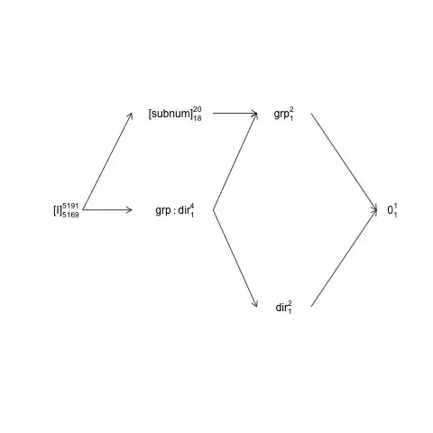
Here random terms are enclosed in brackets, 0 represents the overall mean
(or intercept), [I] represents the error term, the super-script numbers are
the number of levels and the sub-script numbers are the number of degrees of
freedom assuming a balanced design. The diagram indicates that the natural
error term (enclosing error stratum) for group is subnum and
that the numerator df for subnum, which equals the denominator df for group,
is 18: 20 minus 1 df for group and 1 df for the overall mean. A more comprehensive introduction to factor structure diagrams is available in chapter 2 here: https://02429.compute.dtu.dk/eBook.
If the data were exactly balanced we would be able to construct the F-tests from
a SSQ-decomposition as provided by anova.lm. Since the dataset is very-closely balanced we can obtain approximate F-tests as follows:
ANT.2 <- subset(ANT, !error)
set.seed(101)
baseline.shift <- rnorm(length(unique(ANT.2$subnum)), 0, 50)
ANT.2$rt <- ANT.2$rt + baseline.shift[as.numeric(ANT.2$subnum)]
fm <- lm(rt ~ group * direction + subnum, data=ANT.2)
(an <- anova(fm))
Analysis of Variance Table

Response: rt
                  Df   Sum Sq Mean Sq  F value Pr(>F)
group              1   994365  994365 200.5461 <2e-16 ***
direction          1     1568    1568   0.3163 0.5739
subnum            18  7576606  420923  84.8927 <2e-16 ***
group:direction    1    11561   11561   2.3316 0.1268
Residuals       5169 25629383    4958
---
Signif. codes:  0 ‘***’ 0.001 ‘**’ 0.01 ‘*’ 0.05 ‘.’ 0.1 ‘ ’ 1
Here all F and p values are computed assuming that all terms have the residuals as their enclosing error stratum, and that is true for all but 'group'. The 'balanced-correct' F-test for group is instead:
F_group <- an["group", "Mean Sq"] / an["subnum", "Mean Sq"]
c(Fvalue=F_group, pvalue=pf(F_group, 1, 18, lower.tail = FALSE))
   Fvalue    pvalue
2.3623466 0.1416875
where we use the subnum MS instead of the Residuals MS in the F-value
denominator.
Note that these values match quite well with the Satterthwaite results:
model <- lmer(rt ~ group * direction + (1 | subnum), data = ANT.2)
anova(model, type=1)
Type I Analysis of Variance Table with Satterthwaite's method
                 Sum Sq Mean Sq NumDF DenDF F value Pr(>F)
group           12065.3 12065.3     1    18  2.4334 0.1362
direction        1951.8  1951.8     1  5169  0.3936 0.5304
group:direction 11552.2 11552.2     1  5169  2.3299 0.1270
Remaining differences are due to the data not being exactly balanced.
The OP compares anova.lm with anova.lmerModLmerTest, which is ok, but to compare like with like we have to use the same contrasts.
In this case there is a difference between anova.lm and anova.lmerModLmerTest since they produce Type I and III tests by default respectively, and for this dataset there is a
(small) difference between the Type I and III contrasts:
show_tests(anova(model, type=1))$group
               (Intercept) groupTreatment directionright groupTreatment:directionright
groupTreatment           0              1    0.005202759                     0.5013477

show_tests(anova(model, type=3))$group # type=3 is default
               (Intercept) groupTreatment directionright groupTreatment:directionright
groupTreatment           0              1              0                           0.5
If the data set had been completely balanced the type I contrasts would have
been the same as the type III contrasts (which are not affected by the observed
number of samples).
One last remark is that the 'slowness' of the Kenward-Roger method is not due to
model re-fitting, but because it involves computations with the marginal
variance-covariance matrix of the observations/residuals (5191x5191 in this case)
which is not the case for Satterthwaite's method.
Concerning model2
As for model2 the situation becomes more complex and I think it is easier to
start the discussion with another model where I have included the
'classical' interaction between subnum and direction:
model3 <- lmer(rt ~ group * direction + (1 | subnum) +
                 (1 | subnum:direction), data = ANT.2)
VarCorr(model3)
 Groups           Name        Std.Dev.
 subnum:direction (Intercept) 1.7008e-06
 subnum           (Intercept) 4.0100e+01
 Residual                     7.0415e+01
Because the variance associated with the interaction is essentially zero (in the
presence of the subnum random main-effect) the interaction
term has no effect on the calculation of denominator degrees of freedom, F-values and p-values:
anova(model3, type=1)
Type I Analysis of Variance Table with Satterthwaite's method
                 Sum Sq Mean Sq NumDF DenDF F value Pr(>F)
group           12065.3 12065.3     1    18  2.4334 0.1362
direction        1951.8  1951.8     1  5169  0.3936 0.5304
group:direction 11552.2 11552.2     1  5169  2.3299 0.1270
However, subnum:direction is the enclosing error stratum for subnum so if
we remove subnum all the associated SSQ falls back into subnum:direction
model4 <- lmer(rt ~ group * direction +
                 (1 | subnum:direction), data = ANT.2)
Now the natural error term for group, direction and group:direction is
subnum:direction and with nlevels(with(ANT.2, subnum:direction)) = 40 and
four parameters the denominator degrees of freedom for those terms should be
about 36:
anova(model4, type=1)
Type I Analysis of Variance Table with Satterthwaite's method
                 Sum Sq Mean Sq NumDF  DenDF F value  Pr(>F)
group           24004.5 24004.5     1 35.994  4.8325 0.03444 *
direction          50.6    50.6     1 35.994  0.0102 0.92020
group:direction   273.4   273.4     1 35.994  0.0551 0.81583
---
Signif. codes:  0 ‘***’ 0.001 ‘**’ 0.01 ‘*’ 0.05 ‘.’ 0.1 ‘ ’ 1
These F-tests can also be approximated with the 'balanced-correct' F-tests:
an4 <- anova(lm(rt ~ group*direction + subnum:direction, data=ANT.2))
an4[1:3, "F value"] <- an4[1:3, "Mean Sq"] / an4[4, "Mean Sq"]
an4[1:3, "Pr(>F)"] <- pf(an4[1:3, "F value"], 1, 36, lower.tail = FALSE)
an4
Analysis of Variance Table

Response: rt
                   Df   Sum Sq Mean Sq F value Pr(>F)
group               1   994365  994365  4.6976 0.0369 *
direction           1     1568    1568  0.0074 0.9319
group:direction     1    10795   10795  0.0510 0.8226
direction:subnum   36  7620271  211674 42.6137 <2e-16 ***
Residuals        5151 25586484    4967
---
Signif. codes:  0 ‘***’ 0.001 ‘**’ 0.01 ‘*’ 0.05 ‘.’ 0.1 ‘ ’ 1
now turning to model2:
model2 <- lmer(rt ~ group * direction + (direction | subnum), data = ANT.2)
This model describes a rather complicated random-effect covariance structure
with a 2x2 variance-covariance matrix.
The default parameterization is not easy
to deal with and we are better of with a re-parameterization of the model:
model2 <- lmer(rt ~ group * direction + (0 + direction | subnum), data = ANT.2)
If we compare model2 to model4, they have equally many random-effects; 2 for
each subnum, i.e. 2*20=40 in total. While model4 stipulates a single variance
parameter for all 40 random effects, model2 stipulates that each subnum-pair of random effects has a bi-variate normal distribution with a 2x2 variance-covariance matrix the parameters of which are given by
VarCorr(model2)
 Groups   Name           Std.Dev. Corr
 subnum   directionleft  38.880
          directionright 41.324   1.000
 Residual                70.405
This indicates over-fitting, but let's save that for another day. The important point here is that model4 is a special-case of model2 and that model is also a special case of model2. Loosely (and intuitively) speaking (direction | subnum) contains or captures the variation associated with the main effect subnum as well as the interaction direction:subnum. In terms of the random effects we can think of these two effects or structures as capturing variation between rows and rows-by-columns respectively:
head(ranef(model2)$subnum)
  directionleft directionright
1    -25.453576     -27.053697
2     16.446105      17.479977
3    -47.828568     -50.835277
4     -1.980433      -2.104932
5      5.647213       6.002221
6     41.493591      44.102056
In this case these random effect estimates as well as the variance parameter
estimates both indicate that we really only have a random main effect
of subnum (variation between rows) present here.
What this all leads up to is that Satterthwaite denominator degrees of freedom in
anova(model2, type=1)
Type I Analysis of Variance Table with Satterthwaite's method
                 Sum Sq Mean Sq NumDF   DenDF F value Pr(>F)
group           12059.8 12059.8     1  17.998  2.4329 0.1362
direction        1803.6  1803.6     1 125.135  0.3638 0.5475
group:direction 10616.6 10616.6     1 125.136  2.1418 0.1458
is a compromise between these main-effect and interaction structures: The group
DenDF remains at 18 (nested in subnum by design) but the direction and
group:direction DenDF are compromises between 36 (model4) and 5169
(model).
I don't think anything here indicates that the Satterthwaite approximation (or its implementation in lmerTest) is faulty.
The equivalent table with the Kenward-Roger method gives
anova(model2, type=1, ddf="Ken")
Type I Analysis of Variance Table with Kenward-Roger's method
                 Sum Sq Mean Sq NumDF  DenDF F value Pr(>F)
group           12059.8 12059.8     1 18.000  2.4329 0.1362
direction        1803.2  1803.2     1 17.987  0.3638 0.5539
group:direction 10614.7 10614.7     1 17.987  2.1414 0.1606
It is not surprising that KR and Satterthwaite can differ but for all practical purposes the difference in p-values is minute. My analysis above indicates that the DenDF for direction and group:direction should not be smaller than ~36 and probably larger than that given that we basically only have the random main effect of direction present, so if anything I think this is an indication that the KR method gets the DenDF too low in this case. But keep in mind that the data don't really support the (group | direction) structure so the comparison is a little artificial - it would be more interesting if the model was actually supported.

ezAnovawarning as you should not run 2x2 anova if in fact your data are from 2x2x2 design. – Jiri Lukavsky Feb 06 '14 at 17:27ezcould be re-worded; it actually has two parts that are important: (1) that data is being aggregated and (2) stuff about partial designs. #1 is most pertinent to the discrepancy as it explains that in order to do a traditional non-mixed-effects anova, one must aggregate the data to a single observation per cell of the design. In this case, we want one observation per subject per level of the "direction" variable (whilst maintaining group labels for subjects). ezANOVA computes this automatically. – Mike Lawrence May 21 '14 at 17:48summary(aov(rt ~ group*direction + Error(subnum/direction), data=ANT.2))and it gives 16 (?) dfs forgroupand 18 fordirectionandgroup:direction. The fact that there are ~125 observations per group/direction combination is pretty much irrelevant for RM-ANOVA, see e.g. my own question https://stats.stackexchange.com/questions/286280: direction is tested, so-to-say, against subject-direction interaction. – amoeba Jan 05 '18 at 18:41lmerTestthat estimates ~125 dfs. – amoeba Jan 05 '18 at 18:53lmerTest::anova(model2, ddf="Kenward-Roger")returns 18.000 df forgroupand17.987df for the other two factors, which is in excellent agreement with RM-ANOVA (as per ezAnova). My conclusion is that Satterthwaite's approximation fails formodel2for some reason. – amoeba Jan 07 '18 at 14:55