Detecting a single change point within an interval with a certain probability

Question

I have a dataset $D$ of binary values, with length $|D|$. There is some unknown $d \in \left[1,2,\ldots,|D|\right]$ (usually, $d$ will be somewhere in the middle) such that, for any $i<d$, $D_i$ comes from a Bernoulli distribution with success probability $Q_1$, and for $i \geq d$, $D_i$ comes from a Bernoulli distribution with success probability $Q_2$. For the purposes of this question, assume $0 < Q_1 < 1/2 < Q_2 < 1$.

If I use a sliding window of size $k \ll |D|$ and take the sum within the window, I'll find that when the window is only on values with index $i < d$, the sum will hover around $kQ_1$, and when the window is only on values with index $i \geq d$, the sum will hover around $kQ_2$. As the window slides through indices around $i \approx d$, the sum will jump from $kQ_1$ to $kQ_2$, marking a change point. (I'm definitely open to other methods!)

I want to use an algorithm like step detection to detect $d$, but I don't want to appeal to heuristics. I want to find a way to get within some bound of $d$ with at least a certain probability. This problem is easier than the general change point detection problem because there is exactly one change point, and I know the value of the mean before and after $d$ (so I know the magnitude of the change). Is this a known problem? I'm thinking that we can bound the probability of being within some multiple of $k$ from $d$, and that the calculation would involve calculating the probability that you get a sum of $kQ_1$ when the binomial process has $p = Q_2$ and vice versa.

This problem is also similar to this question, though there they also don't seem to get any complexity results.

Answer 1

Let us consider this problem from a Bayesian perspective. We start with a prior distribution on the changepoint, let us say, $d \sim U(\{1, 2, \dots, |D|\})$. Given $d$, the probability of seeing $x_1$ successes from the Bernoulli distribution for $i < d$ and $x_2$ successes from the Bernoulli distribution for $i \geq d$ is:

$$p(x_1,x_2 | Q_1, Q_2, d, |D|) = p(x_1|Q_1, d-1)p(x_2|Q_2,|D|-d+1)$$

where the component distributions on the right-hand side are Binomial distributions. This gives us the likelihood function; given our uniform prior distribution, the posterior distribution of $d$ will be proportional to the likelihood function.

An example in R follows. We set $Q_1 = 0.25$, $Q_2 = 0.75$, $|D| = 100$ and $d = 30$.

Q_1 <- 0.25
Q_2 <- 0.75
x <- c(rbinom(29, 1, Q_1), rbinom(71, 1, Q_2))
lf <- function(d) {
  if (d > 1) {
    x1 <- sum(x[1:(d-1)])
    x2 <- sum(x) - x1
    retval <- dbinom(x1, d-1, Q_1) * dbinom(x2, 101-d, Q_2)
  } else {
    retval <- dbinom(sum(x), 100, Q_2)
  }
  retval
}
posterior <- rep(0,100)
for (d in seq_along(posterior)) {
  posterior[d] <- lf(d)
}
posterior <- posterior / sum(posterior)

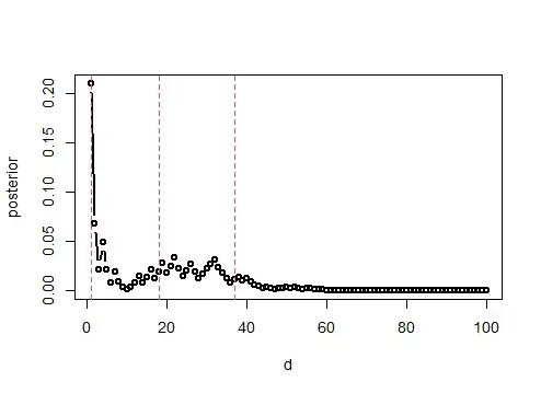
A plot of the posterior distribution, with vertical lines at the cumulative 10th, 50th, and 90th percentiles:

Note, however, that with this little data, this is a good result. If your probabilities are closer together and you don't have many observations, the randomness inherent in the Bernoulli distribution can result in posteriors that look like this (here $Q_1 = 0.35$ and $Q_2 = 0.65$):

The posterior mean is 17.5, and the true value is within the posterior 10%-90% range. Still, the posterior has a mode at $d=1$, thanks to the fact that the sum of the observations is 61, which is quite compatible with the data being drawn from a single Binomial$(100, 0.65)$ distribution.

Of course, we aren't constrained to use a uniform prior on $d$. We now model our belief that the changepoint is more likely to be in the middle of the sample than near the tails using a rescaled $Beta(2,2)$ distribution:

which, applied to the same data that generated the previous posterior, results in: