Logistic regression: restrict the prediction range

Question

I am running a basic logistic regression with a single independent variable (X) and one dependent variable (y). In the accompanying figure, the logistic regression predicts values that tend to 0 and 1 for low and large X values, respectively. However, the probabilities computed from the data tend to be 0.2 and 0.8 for large and small X values.

I am seeking a modified version of the logistic regression that better fits my data and Ideally, I would like a solution that still allows for the interpretation of model results in terms of odds ratios, if possible. Any suggestions?

Answer 1

Logistic regression is actually quite inflexible, since it is linear in the logit, a fact that is somewhat obscured by the fact that the plot on the original scale is nonlinear. In the present case, it tries to fit both in the middle and at the extremes of the predictor, and it's at the extremes that it is visible it's not doing a good job. You rather obviously have a lot of data, at least in this (toy?) example, so you could address the nonlinearity by using a spline transform of the predictor.

However, judging from the blue dots in your graph, you actually simulated data that is not well described by the logit in the first place, since the probabilities are discontinuous. If you have reason to suspect discontinuities, you could certainly model them (but discontinuities rarely happen in nature).

With less data, you can easily overfit using splines, so I would recommend that you do cross-validation to select the number of spline knots, and then are very careful about any inferential statistics you might want to do, but that is already dubious because of your large amount of data.

Answer 2

A logistic regression can do this on its own with the right features, though the decrease in probability seems to be sharp instead of gradual. It really looks like a strict discontinuity at $x=50$, so an indicator of $x>50$ or not might be your best feature, though it is often poor practice to bin continuous variables like this (though this looks like an extreme case).

Answer 3

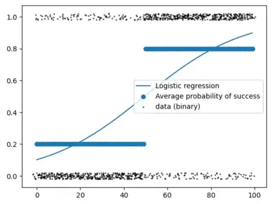
The logistic regression tends toward 0 or 1 because the log-odds of the outcome is linear in the predictor, which (for a positive coefficient, like in your data) causes it to grow without bound as the predictor gets larger, and vice versa when it gets smaller. This is analogous to how ordinary linear regression can produce unreasonable predictions when it extrapolates outside of the values commonly seen in the fitting data.

There are a variety of ways to handle this, but I think the best one is to use a generalized additive model (GAM). A GAM uses a set of flexible basis functions to develop an arbitrary smoothed curve for the linear predictor (i.e., the log-odds in a logistic regression). Here's an example that I whipped up from some data I had lying around.

In this case, the predictor has a "normal" range where the risk of the event is lower than average, and the log-odds adjustment (keep in mind that there is still an intercept term that sets the base rate) increases rapidly once you get out of that range. However, the effect saturates so that you don't get the virtual certainty of an event that you are seeing in your model. Interestingly, the risk saturates at a higher level for high values than for low.

The easiest way to fit GAMs is using the mgcv package for R. I will say that there is a bit of a learning curve for mgcv, so you need to be prepared to do some reading, but it's worth it, as in my experience GAMs produce a very reasonable model for a wide range of real-world phenomena.