How to perform mixed-effect model for data with repeated measurements?

Question

I want to analyze forest regeneration after a forest fire. I have a data frame containing NDVI values (NDVI_mean) (NDVI is a vegetation index for plant vigor) of different study sites (Treatment) over time (date). The study sites are grouped in different management treatments (Management1). This is the head and tail of the data:

   Treatment NDVI_mean       date Management1
1          G 0.7918969 2018-10-11     Control
2          J 0.1899928 2018-10-11    Clearcut
3          H 0.2378630 2018-10-11    Clearcut
4          C 0.3631807 2018-10-11       PR1/2
5          D 0.3294372 2018-10-11       PR1/2
6          E 0.4611494 2018-10-11       PR3/4
7          F 0.3681659 2018-10-11       PR3/4
8          I 0.3020894 2018-10-11    Clearcut
9          B 0.3247002 2018-10-11          NR
10         K 0.3109387 2018-10-11          NR
11         L 0.8071204 2018-10-11     Control
12         G 0.8191044 2018-11-28     Control
13         J 0.1952865 2018-11-28    Clearcut
14         H 0.2209233 2018-11-28    Clearcut
15         C 0.3942993 2018-11-28       PR1/2
16         D 0.3285107 2018-11-28       PR1/2
17         E 0.4192142 2018-11-28       PR3/4
18         F 0.3856550 2018-11-28       PR3/4
19         I 0.2522038 2018-11-28    Clearcut
20         B 0.3300189 2018-11-28          NR
21         K 0.2990551 2018-11-28          NR
22         L 0.8361506 2018-11-28     Control
23         G 0.8274411 2018-12-05     Control
...
479         E 0.5348337 2022-06-15       PR3/4
480         F 0.4959483 2022-06-15       PR3/4
481         I 0.5295775 2022-06-15    Clearcut
482         B 0.4168112 2022-06-15          NR
483         K 0.4540260 2022-06-15          NR
484         L 0.6940871 2022-06-15     Control

I want to test if there are significant differences in NDVI_mean between the different groups (Management1). However, the results of the mixed-effect model I use in lme4 seem a bit off, as they indicate that there are no significant differences between any group except for the control group to others.

This is what I have tried so far:

model <- lmer(NDVI_mean ~ Management1 + (1 | Treatment), data = data_all)
summary(model)
mc <- glht(model, linfct = mcp(Management1 = "Tukey"))
summary(mc)

     Simultaneous Tests for General Linear Hypotheses
Multiple Comparisons of Means: Tukey Contrasts
Fit: lmer(formula = NDVI_mean ~ Management1 + (1 | Treatment), data = data_all)
Linear Hypotheses:
                         Estimate Std. Error z value Pr(>|z|)

Control - Clearcut == 0  0.336027   0.029192  11.511   <1e-04 ***
NR - Clearcut == 0      -0.038349   0.029192  -1.314    0.682

PR1/2 - Clearcut == 0   -0.031177   0.029192  -1.068    0.822

PR3/4 - Clearcut == 0    0.019608   0.029192   0.672    0.962

NR - Control == 0       -0.374376   0.031979 -11.707   <1e-04 ***
PR1/2 - Control == 0    -0.367204   0.031979 -11.483   <1e-04 ***
PR3/4 - Control == 0    -0.316419   0.031979  -9.895   <1e-04 ***
PR1/2 - NR == 0          0.007173   0.031979   0.224    0.999

PR3/4 - NR == 0          0.057957   0.031979   1.812    0.365

PR3/4 - PR1/2 == 0       0.050785   0.031979   1.588    0.504

Signif. codes:  0 ‘*’ 0.001 ‘’ 0.01 ‘*’ 0.05 ‘.’ 0.1 ‘ ’ 1
(Adjusted p values reported -- single-step method)

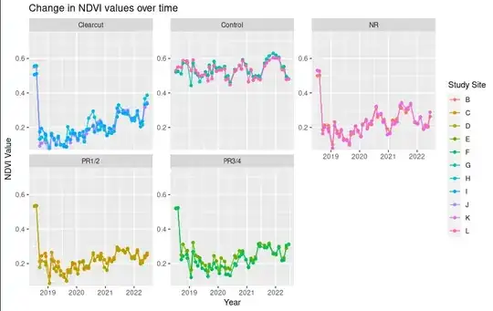
Looking at the plotted data I would expect the differences of some of the groups to be significant:

Plot of my data

I am wondering if I am overseeing something with my code or there are just no significant differences.

EDIT

I should have clarified my research question better in the first place:

I want to analyze, which Management1 group has a stronger effect on NDVI_mean over time.

As a first step, I switched to lme as suggested by Shawn. As I want to evaluate the changes of NDVI_meanover time, this is my code:

model <- lme(NDVI_mean ~ Management1, random = ~1 | date, correlation = corAR1(form = ~ 1 | date), data = Data_2018_2022) With the following output:

Linear mixed-effects model fit by REML
  Data: Data_2018_2022 
        AIC       BIC   logLik
  -1240.825 -1207.452 628.4127
Random effects:
 Formula: ~1 | date
        (Intercept)   Residual
StdDev:  0.07154796 0.05647643
Correlation Structure: AR(1)
 Formula: ~1 | date 
 Parameter estimate(s):
       Phi 
0.09700646 
Fixed effects:  NDVI_mean ~ Management1 
                       Value   Std.Error  DF  t-value p-value
(Intercept)        0.3193368 0.011910976 436 26.81030  0.0000
Management1Control 0.4485332 0.007679661 436 58.40534  0.0000
Management1NR      0.0307109 0.007887175 436  3.89377  0.0001
Management1PR1/2   0.0246634 0.007886995 436  3.12709  0.0019
Management1PR3/4   0.0580982 0.007886995 436  7.36633  0.0000
 Correlation: 
                   (Intr) Mngm1C Mng1NR M1PR1/
Management1Control -0.265

Management1NR      -0.257  0.409

Management1PR1/2   -0.256  0.377  0.366

Management1PR3/4   -0.256  0.377  0.366  0.399
Standardized Within-Group Residuals:
        Min          Q1         Med          Q3         Max 
-3.00833022 -0.53491680 -0.03658359  0.59397622  4.30824733
Number of Observations: 484
Number of Groups: 44

When I plot the normalized residuals plot(ACF(model, resType = "normalized"), alpha = 0.05)

The plot looks like this.

ACF plot

It seems like there is still an autocorrelation. Is my overall approach valid, or am I overseeing something?

EDIT2

I have followed the suggestions of @Edm and fit the model as following: model <- gls(NDVI_mean ~ Management1 + splines::ns(year_month_numeric), correlation = corCAR1(form = ~ year_month_numeric | Treatment), data = Data_2018_2022)

I run into the problem that when I want to include an interaction of Management1 and date Data_2018_2022$Management1_date <- interaction(Data_2018_2022$Management1,Data_2018_2022$year_month_numeric) in the model model <- gls(NDVI_mean ~ Management1_date + splines::ns(year_month_numeric), correlation = corCAR1(form = ~ year_month_numeric | Treatment), data = Data_2018_2022), I get the error Error in glsEstimate(object, control = control) : computed "gls" fit is singular, rank 221

Also, there is still a autocorrelation in the residuals:

Your model doesn't seem to include any evaluation of the changes of NDVI_mean over time. Your plots suggest that, if there are any differences among Management1 values, they are in those patterns over time: PR1/2 is almost flat after the initial drop, while Clearcut seems to rise. Also, your analysis seems to include the initial (pre-intervention?) outcome values, before the big drops, along with all the later values, muddying the comparisons. Look at Frank Harrell's chapter on longitudinal responses, along with Shawn's answer and Robert's comments. — EdM, Jan 11 '24 at 16:22
Your data seem to have a seasonal variation, with peaks particularly noticeable in mid 2020 and mid 2021 in most of the groups. That might account for the residual autocorrelation. The singular fit suggests that you might not have enough data to fit a complicated model. You might need to simplify, e.g.: just use a linear model (no spline) for date and its interaction with Management1, use standard linear regression with robust standard errors instead of a correlation structure to account for the repeated measures. — EdM, Jan 19 '24 at 13:59

score 8 · Answer 1 · answered Jan 11 '24 at 15:34

8

I don't see how this is completely obvious given the plots. The control group on average necessarily has larger values (you can see the this clearly by where the data points are on the y-axis) but the difference is not extreme (on average a .4 difference). It also appears that the study sites don't vary much here.

I will note that because your data has a time-series element to it, that it may be useful to check if there are some serious autocorrelation issues going on here (you'll want to check the normalized residuals in a mixed model). Run an ACF plot and see if the residuals have serious problems. You may need to switch to lme to model that as an ARIMA process. An example can be found here.

Finally, I would advise against chasing statistical significance. You can look through some of my posts here to see why this can be problematic.

answered Jan 11 '24 at 15:34

Shawn Hemelstrand

13,543

3

I agree with Shawn (+1 btw), especially about handling the residual correlation structure appropriately. I would just add that Toeplitz and ante-dependence should also be considered. Check my answer here for further details:Beyond AR(1) as a covariance structure for mixed models with repeated measures. Also, the mmrm package is a fairly new package designed specifically for these kinds of models (repeated measures). – Robert Long Jan 11 '24 at 15:52
Thank you very much, Shawn. I tried switching to lme and edited my question accordingly. – Vik123 Jan 14 '24 at 12:57
@Vik123 as best as I can tell, your syntax doesn't indicate that you specified an autocorrelation model. Try the code from the answer I linked, which includes the argument correlation = corAR1(form = ~ 1 | Treatment) for your autocorrelation structure (if there are equally spaced intervals). I'm less experienced with ARIMA type models but the ACF plot looks abnormal given it simply stops. – Shawn Hemelstrand Jan 14 '24 at 14:41
Thank you for your answer, Shawn. Including the argument you suggested results in following error: Error in lme.formula(NDVI_mean ~ Management1, random = ~1 | date, correlation = corAR1(form = ~1 | : incompatible formulas for groups in 'random' and 'correlation'
As far as I understand, the random variable and the correlation variable must both be the same. When I use correlation = corAR1(form = ~ 1 | date) the model output varies but the SCF plot stays the same.
– Vik123 Jan 14 '24 at 15:52
I'm confused. Why is the random effect "treatment" in your original model but it is listed as "date" in the second model? I also realize now why your ACF plot is weird, you set the mag lax to 78, which I'm assuming is from the linked answer. You don't need to do this in your case. – Shawn Hemelstrand Jan 14 '24 at 21:22
@ShawnHemelstrand I have changed the random effect from Treatment to date because after thinking about it, it appears to make more sense since the Treatment variable is a combination of Management1, Management2 and Management3 (which I did not include in my example data. I edited my initial post once again. – Vik123 Jan 15 '24 at 10:59
Check out the answer from EdM. – Shawn Hemelstrand Jan 16 '24 at 01:10

score 2 · Answer 2 · answered Jan 15 '24 at 15:37

It doesn't make sense to treat date as the random-effect term, as in your second model; that doesn't account for the actual ordering of date values. That second model also doesn't account for the correlations within each level of Treatment, as that's been removed. Furthermore, the plots suggest that the very first observation in all cases is a pre-intervention value, while your code implicitly includes them with the NDVI_mean post-intervention values.

Chapter 7 of Frank Harrell's Regression Modeling Strategies discusses ways to model such longitudinal data. Briefly: include the pre-intervention value as a predictor in the model; model date continuously but flexibly; account for the correlations within each "subject" (the various Treatment values in your situation).

One recommendation is generalized least squares, e.g. via gls() from the nlme package you are now using or the Gls() function of Harrell's rms package, which is convenient for post-modeling analysis. Generalized least squares can handle several different correlation structures in time. An extended example in that chapter shows how to build such a model and use variograms to evaluate your choice of structure.

You would include Management1 as a fixed predictor. If you wanted to examine whether the trajectory with respect to date differs among values of Management1, you would include a corresponding interaction term between Management1 and date.

Thank you very much for your answer, @EdM. The link you provided is quite incomprehensible for my level of statistics. Could you maybe elaborate on how to model date continuously but flexible? I tried to look it up without success. All I could come up with is splines::ns(date).
I have now removed the pre-intervention value from the data to simplify it a bit.

With accounting for correlations within each subject do you mean correlation = corAR1(form = ~1 | Treatment) ? — Vik123, Jan 16 '24 at 10:13
@Vik123 a regression spline like ns() is what I had in mind. corAR1 might work if all observations are equally spaced, in order in the data, and are complete for all cases. For correlations over time it can be safer to use a continuous-time structure and specify the time covariate in form. For example, the Harrell reference with your data might suggest corCAR1(form=~date|Treatment) or some other continuous-time structure like corExp,corLin,corGaus,or corSpher. Make sure your date values are converted to numeric or interpreted internally as members of the Date class. — EdM, Jan 16 '24 at 14:05
I have tried to follow your suggestions and fit the model as model <- gls(NDVI_mean ~ Management1 + splines::ns(year_month_numeric), correlation = corCAR1(form = ~ year_month_numeric | Treatment), data = Data_2018_2022). I have tried to put Data_2018_2022$Management1_date <- interaction(Data_2018_2022$Management1, Data_2018_2022$year_month_numeric) into the model but get the error Error in glsEstimate(object, control = control) : computed "gls" fit is singular, rank 221. I will update my question accordingly. — Vik123, Jan 19 '24 at 08:40

How to perform mixed-effect model for data with repeated measurements?

2 Answers2

Linked