$\chi^2$-distribution of $(x_1-x_2+x_3+x_4)^2-(-x_1+x_2+x_3+x_4)^2$ with $x_i \sim N(\mu_i,\sigma_i)$

Question

Given are 4 independent normal variables $x_i \sim \mathcal{N}(\mu_i,\sigma_i)_{i=1,\ldots,4}$, that are used to define the random variable $$Z\sim (x_1 - x_2 + x_3 + x_4)^2 - (-x_1 + x_2 + x_3 + x_4)^2.\tag{1}$$

Each squared term in eq.(1) is a linear combination of independent normal variables, whence each of those squares has a noncentral $\chi^2(k,M)$-distribution with $k=1$ degree of freedom and noncentrality parameter $M$. The two linear combinations are also orthogonal, $\begin{pmatrix} 1 & -1 & 1&1 \end{pmatrix} \cdot \begin{pmatrix} -1 & 1 & 1&1 \end{pmatrix}^T =0$ , whence uncorrelated; and because they are uncorrelated joint random variables, they are independent (see here).

Thus the squared linear combinations in eq.(1) can be written as a difference of $\chi^2$-variables $$Z\sim s \left( \chi^2\left(1,M_1\right)- \chi^2\left(1,M_2\right)\right)\tag{2}$$

with noncentrality parameters $M_1=\dfrac{1}{s}\left(\mu_1-\mu_2+\mu_3+\mu_4\right)^2, M_2=\dfrac{1}{s}\left(-\mu_1+\mu_2+\mu_3+\mu_4\right)^2$ and total variance $s=\sum_{i=1}^4\sigma^2_i$.

However this approach only works, if all $\sigma_i$ are identical. How to express eq.(1) by $\chi^2$-variables for different $\sigma_i$?

Graphical examples for PDF

All $\sigma_i$ are identical.

$\sigma=(5,5,5,5), \mu=(2,-11,-1,4)$, black: eq(1), red: eq(2) (both plots almost overlap)

All $\sigma_i$ are different.

$\sigma=(5,4,3,2), \mu=(2,-11,-1,4)$, black: eq(1), red: eq(2)

Answer 1

This problem is initially written as the difference in the squares of two correlated normals.

$$Z=(X_1-X_2+X_3+X_4)^2-(-X_1+X_2+X_3+X_4)^2$$

where all of the $X_i$ are independent random variables with potentially different means and variances: $X_i \sim N(\mu_i,\sigma_i^2)$.

The request is to re-write $Z$ in terms of the difference in two independent noncentral chisquare random variables times some constant:

$$Z=s(W_1-W_2)$$

where $W_i\sim \chi^2(1,m_i)$. To do so we do something similar to the idea presented in @whuber 's comment: The characteristic functions are found for both characterizations of $Z$ and then we equate all of the coefficients for the characteristic function argument $t$.

To have a less cluttered expression for

$$Z=(X_1-X_2+X_3+X_4)^2-(-X_1+X_2+X_3+X_4)^2$$

we first re-write $Z$ as follows:

$$Z=(Z_{12}+Z_{34})^2 - (-Z_{12}+Z_{34})^2$$

where $Z_{12}=X_1-X_2$ and $Z_{34}=X_3+X_4$. $Z_{12}$ and $Z_{34}$ are independent normals with respective means and variances $\mu_{12}=\mu_1-\mu_2$, $\mu_{34}=\mu_3+\mu_4$, $\sigma_{12}^2=\sigma_1^2+\sigma_2^2$, and $\sigma_{34}^2=\sigma_3^2+\sigma_4^2$.

Written this way the characteristic function of $Z$ is found with

Format[μ[i_]]:=Subscript[μ,i]
Format[σ[i_]]:=Subscript[σ,i]
dist = TransformedDistribution[(z[12] + z[34])^2 - (-z[12] + z[34])^2,
    {z[12] \[Distributed] NormalDistribution[μ[12], σ[12]],
     z[34] \[Distributed] NormalDistribution[μ[34], σ[34]]}];
cf = CharacteristicFunction[dist, t]

$$\frac{e^ {-\frac{4 t \left(-i \mu _{12} \mu _{34}+2 \mu _{34}^2 \sigma _{12}^2 t+2 \mu _{12}^2 \sigma _{34}^2 t\right)}{16 \sigma _{12}^2 \sigma _{34}^2 t^2+1}}}{\sqrt{16 \sigma _{12}^2 \sigma _{34}^2 t^2+1}}=\frac{e^{\frac{-t^2 \left(8 \mu _{34}^2 \sigma _{12}^2+8 \mu _{12}^2 \sigma _{34}^2\right)+i 4 \mu _{12} \mu _{34} t}{16 \sigma _{12}^2 \sigma _{34}^2 t^2+1}}}{\sqrt{16 \sigma _{12}^2 \sigma _{34}^2 t^2+1}}$$

The characteristic function for the alternate formulation is found with the following:

Format[m[i_]]:=Subscript[m,i]
dist2 = TransformedDistribution[s (w[1] - w[2]),
   {w[1] \[Distributed] NoncentralChiSquareDistribution[1, m[1]],
    w[2] \[Distributed] NoncentralChiSquareDistribution[1, m[2]]}];
cf2 = CharacteristicFunction[dist2, t];

$$\frac{e^{-s t \left(\frac{m_1}{2 s t+i}+\frac{m_2}{2 s t-i}\right)}}{\sqrt{4 s^2 t^2+1}}=\frac{e^{\frac{-2 \left(m_1+m_2\right) s^2 t^2+i \left(m_1-m_2\right) s t}{4 s^2 t^2+1}}}{\sqrt{4 s^2 t^2+1}}$$

We can find the matching terms of $t$ and $t^2$ in the exponents to determine $m_1$, $m_2$, and $s$. This means we need to simultaneously solve

$$16 \sigma^2_{12} \sigma^2_{34}=4s^2$$ $$8 \mu^2_{34}\sigma^2_{12}+8\mu^2_{12}\sigma^2_{34}=2s^2(m_1+m_2)$$ $$4\mu_{12}\mu_{34}=s(m_1-m_2)$$

sol = Solve[{16 σ[12]^2 σ[34]^2 == 4 s^2, 
  8 μ[34]^2 σ[12]^2 + 8 μ[12]^2 σ[34]^2 == 2 s^2 (m[1] + m[2]), 
  4 μ[12] μ[34] == s (m[1] - m[2])}, {s, m[1], m[2]}]

This results in two solutions:

$$s= \pm 2 \sigma _{12} \sigma _{34}$$ $$m_1= \frac{\left(\mu _{34} \sigma _{12}\pm\mu _{12} \sigma _{34}\right){}^2}{2 \sigma _{12}^2 \sigma _{34}^2}$$ $$m_2= \frac{\left(\mu _{34} \sigma _{12}\mp\mu _{12} \sigma _{34}\right){}^2}{2 \sigma _{12}^2 \sigma _{34}^2}$$

Finally, we can plug in the original parameters:

parms = {μ[12] -> μ[1] - μ[2], μ[34] -> μ[3] + μ[4], σ[12] -> Sqrt[σ[1]^2 + σ[2]^2],  σ[34] -> Sqrt[σ[3]^2 + σ[4]^2]}
sol = sol //. parms

$$s= \pm 2 \sqrt{\sigma _1^2+\sigma _2^2} \sqrt{\sigma _3^2+\sigma _4^2}$$ $$m_1= \frac{\left(\left(\mu _2-\mu _1\right) \sqrt{\sigma _3^2+\sigma _4^2}\pm\left(\mu _3+\mu _4\right) \sqrt{\sigma _1^2+\sigma _2^2}\right){}^2}{2 \left(\sigma _1^2+\sigma _2^2\right) \left(\sigma _3^2+\sigma _4^2\right)}$$ $$m_2= \frac{\left(\left(\mu _1-\mu _2\right) \sqrt{\sigma _3^2+\sigma _4^2}\mp \left(\mu _3+\mu _4\right) \sqrt{\sigma _1^2+\sigma _2^2}\right){}^2}{2 \left(\sigma _1^2+\sigma _2^2\right) \left(\sigma _3^2+\sigma _4^2\right)}$$

As a check consider one of the given examples.

parms = {μ[1] -> 2, μ[2] -> -11, μ[3] -> -1, μ[4] -> 4, σ[1] -> 5,
  σ[2] -> 4, σ[3] -> 3, σ[4] -> 2};
parms1 = {μ[12] -> μ[1] - μ[2], μ[34] -> μ[3] + μ[4], σ[12] -> Sqrt[σ[1]^2 + σ[2]^2],
  σ[34] -> Sqrt[σ[3]^2 + σ[4]^2]};
z1 = RandomVariate[dist /. parms1 /. parms, 1000000];
dist2 = TransformedDistribution[
  s (w[1] - w[2]) /. sol[[2]] /. parms1 /. parms, 
  {w[1] [Distributed] NoncentralChiSquareDistribution[1, m[1]], 
   w[2] [Distributed] NoncentralChiSquareDistribution[1, m[2]]} /. sol[[2]] /. parms1 /. parms];
z2 = RandomVariate[dist2 /. parms, 1000000];
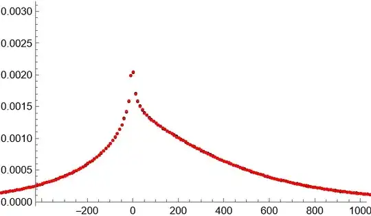
Histogram[z1, "FreedmanDiaconis", "PDF"]

Histogram[z2, "FreedmanDiaconis", "PDF"]

We can also check on the corresponding sample means and variances:

{Mean[#], Variance[#]} & /@ {z1, z2}
(* {{156.019, 49649.8}, {156.27, 49587.}} *)

The pdf can also be easily found numerically using the characteristic function for specified values of the parameters.

Answer to a comment below:

It was asked to find the distribution and characteristic function of a more complicated random variable:

$$X=(z_5-z_3)(z_2-z_4)-(z_1-z_3)(z_6-z_4)$$

Rather than directly using that definition, it appears that Mathematica needs a little help.

First determine the multivariate normal distribution of the 4 differences in normal random variables.

dist = TransformedDistribution[{z[5] - z[3], z[2] - z[4], z[1] - z[3], z[6] - z[4]},
  {z[1] \[Distributed] NormalDistribution[μ[1], σ[1]], 
   z[2] \[Distributed] NormalDistribution[μ[2], σ[2]], 
   z[3] \[Distributed] NormalDistribution[μ[3], σ[3]], 
   z[4] \[Distributed] NormalDistribution[μ[4], σ[4]], 
   z[5] \[Distributed] NormalDistribution[μ[5], σ[5]], 
   z[6] \[Distributed] NormalDistribution[μ[6], σ[6]]}]
(*  MultinormalDistribution[{-μ[3] + μ[5], μ[2] - μ[4], μ[1] - μ[3], -μ[4] + μ[6]}, 
  {{σ[3]^2 + σ[5]^2, 0,               σ[3]^2,           0}, 
   {0,               σ[2]^2 + σ[4]^2, 0,                σ[4]^2}, 
   {σ[3]^2,          0,               σ[1]^2 + σ[3]^2,  0}, 
   {0,               σ[4]^2,          0,                σ[4]^2 + σ[6]^2}}]*)

Now set up rules such that the parameters in the above distribution each have a single symbol. This seems to be necessary for Mathematica to complete in a reasonable amount of time.

parms1 = {-μ[3] + μ[5] -> μ1, μ[2] - μ[4] -> μ2, μ[1] - μ[3] -> μ3, -μ[4] + μ[6] -> μ4,
  σ[3]^2 + σ[5]^2 -> v1, σ[2]^2 + σ[4]^2 -> v2, σ[1]^2 + σ[3]^2 -> v3, 
  σ[4]^2 + σ[6]^2 -> v4, σ[3]^2 -> v5, σ[4]^2 -> v6};
(* Find distribution and characteristic function of the simplified difference 
   of the products of normally distributed random variables *)
dist2 = TransformedDistribution[x[1] x[2] - x[3] x[4],
  {x[1], x[2], x[3], x[4]} [Distributed] dist] /.parms1;
AbsoluteTiming[cf = CharacteristicFunction[dist2, t]]

The result is messy and takes about 4 minutes to run. Now replace with the original parameters:

parms2 = parms1 /. {Rule[a_, b_] -> Rule[b, a]}
cf = cf /. parms2

That result is even messier so I won't show it here.

Answer 2

For this special case the random variable $Z$ can be simplified to the product of two independent normals:

Let $Z_1=4(X_1-X_2)$ and $Z_2=X_3+X_4$. $Z_1$ and $Z_2$ are independent normals with respective means $4(\mu_1-\mu_2)$ and $\mu_3+\mu_4$ and respective variances $16(\sigma_1^2+\sigma_2^2)$ and $\sigma_3^2+\sigma_4^2$. Now

$$Z=(Z_1/4+Z_2)^2-(-Z_1/4+Z_2)^2=Z_1 Z_2$$

Finding moments of $Z$ should be straightforwared. To plot the pdf of $Z$ using Mathematica (which your profile says you have access), one can execute the following:

(* Numerical estimate of the pdf of Z *)
pdf[z_?NumericQ, μ1_?NumericQ, σ1_?NumericQ, μ2_?NumericQ, σ2_?NumericQ] := 
 NIntegrate[PDF[NormalDistribution[μ1, σ1], x] PDF[NormalDistribution[μ2, σ2], z/x]/Abs[x],
 {x, -∞, ∞}]
(* Parameters from your example *)
σz1 = Sqrt[16 (25 + 16)]
σz2 = Sqrt[9 + 4]
μz1 = 4 (2 - (-11))
μz2 = -1 + 4
(* Plot of density *)
Plot[pdf[z, μz1, σz1, μz2, σz2], {z, -400, 1000}]

Expressing Z as a linear combination of two independent noncentral chisquare rv's

Define the distribution of the linear combination.

$$Z=a_1\chi^2(1,m_1)+a_2\chi^2(1,m_2)$$

dist = TransformedDistribution[a1 y1 + a2 y2,
   {y1 \[Distributed] NoncentralChiSquareDistribution[1, m1], 
    y2 \[Distributed] NoncentralChiSquareDistribution[1, m2]}];

Define the distribution of Z expressed as the product of two independent normal rv's.

distz1z2 = TransformedDistribution[z1 z2,
  {z1 \[Distributed] NormalDistribution[μz1, σz1], 
   z2 \[Distributed] NormalDistribution[μz2, σz2]}];

If we can characterize $Z$ as a linear combination of two independent noncentral $\chi^2$ rv's which has 4 parameters, then the first 4 moments need to match with that of the characterization of $Z$ as the product of two independent normals.

sol = Solve[{Mean[distz1z2] == Mean[dist], 
     Variance[distz1z2] == Variance[dist],
     Moment[distz1z2, 3] == Moment[dist, 3], 
     Moment[distz1z2, 4] == Moment[dist, 4]},
    {a1, a2, m1, m2}][[1]] // FullSimplify

From above we know that

parms2 = {σz1 -> Sqrt[16 (σ1^2 + σ2^2)], σz2 -> Sqrt[σ3^2 + σ4^2], 
  μz1 -> 4 (μ1 - μ2), μz2 -> μ3 + μ4};

So in terms of the original parameters the parameters of the linear combination of independent noncentral chisquare rv's are

sol /. parms2

As a minimal check, consider your example.

parms = {μ1 -> 2, μ2 -> -11, μ3 -> -1, μ4 -> 4, σ1 -> 5, σ2 -> 4, σ3 -> 3, σ4 -> 2};
zA = RandomVariate[distz1z2 /. sol /. parms2 /. parms, 1000000];
zB = RandomVariate[dist /. sol /. parms2 /. parms, 1000000];
Histogram[zA, "FreedmanDiaconis", "PDF", PlotRange -> {{-700, 1300}, {0, 0.003}}]

Histogram[zB, "FreedmanDiaconis", "PDF", PlotRange -> {{-700, 1300}, {0, 0.003}}]

Answer 3

This answer only explains why the approach fails but does not say how to get the expected result.

Set $$y_i\sim \mathcal{N}\left(\dfrac{\mu_i}{\sigma_i},1\right)$$ and write $$Z\sim(\sigma_1 y_1-\sigma_2 y_2+\sigma_3 y_3+\sigma_4 y_4)^2-(-\sigma_1 y_1+ \sigma_2 y_2+\sigma_3 y_3+\sigma_4 y_4)^2.$$ You see that the linear combinations are not orthogonal but dependent. They are independent only for the special case $\sigma^2_1+\sigma^2_2=\sigma^2_3+\sigma^2_4$.