An interesting observation regarding the log transformation of data

Question

I stumbled upon something interesting while attempting to do a log transformation for some data (with zeros) today. It seems that there must be a good reason for this that I'm just not seeing. I'm hoping somebody can explain this in an illuminating way. This post has some good answers, but doesn't quite get at this.

I encourage you to read the whole post before giving an answer, but the tldr is basically

If $y_i = \log(x_i+\epsilon)$ and $z_i = \frac{y_i-\bar y}{S_y}$, then the the log likelihood (assuming standard normals) $\sum_{i=1}^n\log\phi(z_i)$ seems to be invariant of $\epsilon$, where $\phi$ is the standard normal pdf.

The question, of course is why does this happen?

Edit

The excellent answer by @MattF does show why this happens. But to me, it's still curious that this occurs for the normal distribution but not for other distributions. Also, it seems obvious (from the plots for example) that the choice of $\epsilon$ makes a huge difference on the shape of the distribution and I assumed (incorrectly, apparently) that this would show up in the log likelihood evaluation. I feel like there is a deeper connection to be made, so I will wait a few days before accepting an answer.

---

For illustration let's make some data with a single problematic zero

set.seed(42)
X <- rgamma(1000, 1.2, 1.2)
m <- min(X)
X <- X - m
hist(X, breaks=30, freq=FALSE, xlim=c(-m, max(X)))
curve(dgamma(x+m, 1.2, 1.2), add=TRUE, lwd=2, col='orange')

Because of this zero, we can't do a log transformation of the data unless we add a constant, ensuring the shifted variables are positive $$y_i = \log(x_i + \epsilon).$$ How to choose $\epsilon$ becomes the natural question. Clearly, the choice of $\epsilon$ matters a great deal. To show this, lets consider two values $\epsilon_1=0.2$ and $\epsilon_2 = 10$.

eps1 <- 0.2
y1 <- log(X + eps1)
z1 <- (y1 - mean(y1))/sd(y1)
eps2 <- 10
y2 <- log(X + eps2)
z2 <- (y2 - mean(y2))/sd(y2)
hist(z1, breaks=30, freq=FALSE)
curve(dnorm(x), add=TRUE, lwd=2, col='orange')
hist(z2, breaks=30, freq=FALSE)
curve(dnorm(x), add=TRUE, lwd=2, col='orange')
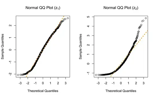
qqnorm(z1, main=expression(paste("Normal QQ Plot (", z[1], ")")))
abline(0, 1, lwd=3, lty=3, col='orange')
qqnorm(z2, main=expression(paste("Normal QQ Plot (", z[2], ")")))
abline(0, 1, lwd=3, lty=3, col='orange')

Clearly the first value of $\epsilon$ is a better choice. To choose an "optimal value", I thought I would choose the value that maximizes the log likelihood $$\sum_{i=1}^n\log \phi(z_i).$$ To my surprise this sum is equal for all values of $\epsilon$, even though the terms of the sum vary drastically.

# LOG LIKELIHOOD FOR EPS1
> sum(log(dnorm(sort(z1))))
[1] -1418.439
LOG LIKELIHOOD FOR EPS2
> sum(log(dnorm(sort(z2))))
[1] -1418.439
THEY ARE EQUAL (UP TO MACHINE PRECISION)
> sum(log(dnorm(sort(z1)))) == sum(log(dnorm(sort(z2))))
[1] TRUE

Although we are now officially treading into "beyond the scope of the problem" waters, for curious parties, I found the value of $\epsilon$ that led to the best qq plot. This can be done with the following R code

qq_func <- function(eps, xx){
  res <- rep(NA, length(eps))
  for(i in seq_along(eps)){
    yy <- log(xx + eps[i])
    zz <- (yy - mean(yy))/sd(yy)
    qq <- qqnorm(zz, plot.it=FALSE)
    res[i] <- sd(qq$x-qq$y)
  }
  return(res)
}
eps_hat <- optim(1.5e-5, llfunc, 
                 method="Brent", lower=0.1, upper=0.5, 
                 xx=X)$par
curve(qq_func(x, xx=X), from=0.1, to=0.5, lwd=2,
      xlab=expression(epsilon), ylab="|qq error|")

This gives an optimal value of $\epsilon = 0.2027$ which is what I'm using moving forward.

---

In summary... the main question is why is evaluation of the log likelihood invariant of $\epsilon$? Although it is secondary, I am also interested in alternatives to the qq plot based approach, but was unable to find any relevant literature or methodology.

Answer 1

This is independent of $\epsilon$ because it’s independent of the $y$’s entirely, and depends only on $n$. Assuming that $S_y$ means $\sqrt{\sum(y_i-\bar{y})^2/(n-1)}$: \begin{align} \log\phi(z) &=\frac{-1}{2}(\ln(2\pi)+z^2)\\ \sum \log\phi(z_i) &=\frac{-1}{2}(n\ln(2\pi)+\sum z_i^2)\\ &=\frac{-1}{2}(n\ln(2\pi)+\sum \frac{(y_i-\bar{y})^2}{S_y^2})\\ &=\frac{-1}{2}(n\ln(2\pi)+n-1) \end{align}

Answer 2

As already implied by other answers, this holds under more general conditions.

Specifically, the result is not a property of the Normal density solely. Neither does it depend on log-transforming the underlying variable $y_i$. To obtain it the following two conditions are sufficient:

1. P1: That the density $f$ we use satisfies a specific differential equation, $f'(z) = \pm zf(z)$, which is indeed satisfied by the Normal density, but not only, see the post https://stats.stackexchange.com/a/311958/28746

2. P2: That the variable $z_i$ that enters the density is "standardized" already in the sample, namely that it has been centered at its sample mean and divided by its sample standard deviation, so as to have zero-mean and unitary sample variance.

PROOF

If the log-likelihood is invariant to $\epsilon$ it must be the case that, $\forall\,\epsilon$,

$$\frac{\partial \sum_{i=1}^n\ln f(z_i)}{\partial \epsilon} = 0 \implies \sum_{i=1}^n \frac{f'(z_i)}{f(z_i)}\frac{\partial z_i}{\partial \epsilon}=0.$$

Given P1, this becomes

$$\sum_{i=1}^n z_i\frac{\partial z_i}{\partial \epsilon}=0.$$

In matrix algebra terms, this is described as "the vector $\{z_i\}$ is orthogonal to the vector $\{\partial z_i/\partial \epsilon\}$."

Is it ?

Given P2, no matter what the $y_i$'s are originally, and no matter how $\epsilon$ affects $y_i$, the resulting $\{z_i\}$ vector will have sample mean zero and unitary sample variance.

This means that

$${\rm P2}:\;s^2_z = \frac 1n \sum_{i=1}^n z_i^2 = 1 \implies \sum_{i=1}^n z_i^2 = n.$$ It follows that

$$\frac{\partial \sum_{i=1}^n z_i^2}{\partial \epsilon} = 0 \implies 2\sum_{i=1}^n z_i\frac{\partial z_i}{\partial \epsilon} = 0.$$

So we obtain orthogonality and the invariance of the log-likelihood under P1 and P2.

These are sufficient conditions. Other sets of conditions may lead to the same result, as the OP appears to have found in relation to the Laplace distribution, that they mention in a comment to another answer (where the standardization that the $z_i$'s incorporate, is done by the median and the mean absolute deviation from the median, respectively). It would appear that in that case too, similar properties drive the result (density such as its log leads to the naked variable, and some notion of standardization that leads to orthogonality).

Answer 3

For the standard normal, the log likelihood is just negative sum of squares plus a constant. Since you've standardized z by the mean + sd of $y$, this is always going to be a constant as a function of $n$ (nothing to do with logs or $\epsilon$'s).

Answer 4

The phenomenon you observe can also be explained through the concept of sufficient statistic.

Basically, some probability distributions have the interesting property that they admit a small number of estimates (called a statistic) such that no further information can be obtained from the same sample regarding the value of a parameter of interest. If a given distributions admits a sufficient statistic $T(X)$ for a parameter $\theta$ (which can be a vector), then the probability density of an i.i.d. data sample $X=[X_1,\dots,X_n]$ can be factorised as $f_{X}(x)=h(x)\,g(\theta ,T(x))$. For example, for the Normal distribution, a sufficient statistic for $[\mu ,\sigma ^{2}]$ is $T(X)=\big[\sum_{i=1}^{n}X_{i},\sum_{i=1}^{n}X_{i}^2\big]$. This means that for the purpose of estimating $\mu$ and $\sigma^{2}$, e.g. through maximum likelihood, $T(X)$ contains all the required information about the data sample $X$. In other words you can distort the data sample $X$ as much as you like but as long as $\sum_{i=1}^{n}X_{i}$ and $\sum_{i=1}^{n}X_{i}^2$ don't change, then the estimated $\mu$ and $\sigma^{2}$ will be the same. This is because in the factorised density above $g(\theta ,T(x))$ depends on $X$ only through $T(X)$ while the factor $h(x)$ (which depends on the data) is irrelevant for the maximisation of $f_{X}(x)$ w.r.t. $\theta$.

If a distribution admits a sufficient statistic w.r.t. to a parameter such that $h(x)$ does not depend on $x$, then $f_{X}(x)=h()\,g(\theta ,T(x))$. In this case the whole density depends on the sample $X$ only through $T(x)$. As you can see in this table, several common distributions have this property, including the Normal distribution. This explains why in your case the density is the same after the log-transformation: because you are rescaling your data so that $T(X)=[0,n-1]$ regardless of the transformation. Another example is the Gamma distribution, which has $h(x)=1$ and $T(X)=\big[\sum_{i=1}^{n}\log(X_{i}),\sum_{i=1}^{n}X_{i}\big]$. In this case you could apply any transformation as you like to your sample and, as long as you manage to keep $\sum_{i=1}^{n}\log(X_{i})$ and $\sum_{i=1}^{n}X_{i}$ the same (which may be non-trivial), the density will be unaffected by such transformations.

---

Example of how any z-scored data sample of length 1000 has a log density for the standard normal distribution which is equal to your example (-1418.439, i.e. $-\frac{n}{2}\log(2\pi) - \frac{n-1}{2}$):

y2 <- rbinom(1000, 1, 0.84)
z2 <- (y2 - mean(y2))/sd(y2)
sum(log(dnorm(sort(z2))))
[1] -1418.439

Try it online!