I want to fit a beta regression with an scaled continuous predictor, and express the slope in terms of proportion (not at the transformed, log-odds scale). In other words, I would like to express the change in the response variable (a proportion), when the predictor increases 1 standard deviation from the mean.
I can get the slope at the probability scale with the emmeans::emtrends() function, but I don't know how to do it manually from the model output. In contrast, I can back-transform and interpret intercepts and factor coefficients manually, or so I think. The fact that I cannot do the same for an scaled continuous predictor suggests I don't understand my model very well. Can anyone shed light on this?
I have found some inspiration in previous questions here, here and here.
See below a reproducible example, showing manual calculation of intercepts, factor coefficients, and slopes.
Note that emmeans::emtrends() appears to take the scaling into account only when it is done in the input data, not on the model formula.
library(betareg)
library(effects)
#> Loading required package: carData
#> lattice theme set by effectsTheme()
#> See ?effectsTheme for details.
library(emmeans)
library(glmmTMB)
library(tidyverse)
#> Warning: package 'ggplot2' was built under R version 4.2.2
#> Warning: package 'tibble' was built under R version 4.2.3
#> Warning: package 'tidyr' was built under R version 4.2.3
#> Warning: package 'purrr' was built under R version 4.2.3
#> Warning: package 'dplyr' was built under R version 4.2.3
#> Warning: package 'stringr' was built under R version 4.2.3
library(visreg)
######### Dataset
data("FoodExpenditure", package = "betareg")
FoodExpenditure$resp <- FoodExpenditure$food / FoodExpenditure$income
FoodExpenditure$income.s <- as.numeric(scale(FoodExpenditure$income))
summary(FoodExpenditure)
#>       food            income         persons           resp

#>  Min.   : 7.431   Min.   :25.91   Min.   :1.000   Min.   :0.1075

#>  1st Qu.:11.069   1st Qu.:42.12   1st Qu.:2.000   1st Qu.:0.2269

#>  Median :14.831   Median :60.45   Median :3.000   Median :0.2611

#>  Mean   :15.953   Mean   :58.44   Mean   :3.579   Mean   :0.2897

#>  3rd Qu.:19.102   3rd Qu.:76.79   3rd Qu.:5.000   3rd Qu.:0.3469

#>  Max.   :28.980   Max.   :88.23   Max.   :7.000   Max.   :0.5612

#>     income.s

#>  Min.   :-1.6326

#>  1st Qu.:-0.8192

#>  Median : 0.1007

#>  Mean   : 0.0000

#>  3rd Qu.: 0.9206

#>  Max.   : 1.4945
######### The back-transformed intercept from a null model coincides with the sample mean
mean(FoodExpenditure$resp)
#> [1] 0.2896702
summary(glmmTMB(resp ~ 1, data = FoodExpenditure, family = beta_family(link = "logit"), dispformula = ~ 1))
#>  Family: beta  ( logit )
#> Formula:          resp ~ 1
#> Data: FoodExpenditure
#>
#>      AIC      BIC   logLik deviance df.resid
#>    -66.7    -63.4     35.3    -70.7       36
#>
#>
#> Dispersion parameter for beta family (): 20.9
#>
#> Conditional model:
#>             Estimate Std. Error z value Pr(>|z|)

#> (Intercept)  -0.8925     0.0763   -11.7   <2e-16 ***
#> ---
#> Signif. codes:  0 '*' 0.001 '' 0.01 '*' 0.05 '.' 0.1 ' ' 1
plogis(- 0.8925)
#> [1] 0.2905942
######### Factors: back-transformed coefficients coincide with raw probabilities calculated from the data
mod.factor <- glmmTMB(resp ~ factor(persons), data = FoodExpenditure, family = beta_family(link = "logit"), dispformula = ~ 1)
summary(mod.factor)
#>  Family: beta  ( logit )
#> Formula:          resp ~ factor(persons)
#> Data: FoodExpenditure
#>
#>      AIC      BIC   logLik deviance df.resid
#>    -66.4    -53.3     41.2    -82.4       30
#>
#>
#> Dispersion parameter for beta family (): 28.5
#>
#> Conditional model:
#>                  Estimate Std. Error z value Pr(>|z|)

#> (Intercept)      -1.06718    0.20873  -5.113 3.17e-07 ***
#> factor(persons)2 -0.09564    0.25723  -0.372  0.71003

#> factor(persons)3  0.21242    0.25180   0.844  0.39889

#> factor(persons)4 -0.01733    0.28018  -0.062  0.95068

#> factor(persons)5  0.26137    0.25112   1.041  0.29796

#> factor(persons)6  0.77294    0.29930   2.582  0.00981 **
#> factor(persons)7  0.45845    0.34230   1.339  0.18046

#> ---
#> Signif. codes:  0 '*' 0.001 '' 0.01 '*' 0.05 '.' 0.1 ' ' 1
Raw probabilities from the data
FoodExpenditure %>% group_by(persons) %>% summarise(mean = mean(food/income)) %>% pull(mean)
#> [1] 0.2491281 0.2317299 0.2947887 0.2564000 0.3130861 0.4256767 0.3675447
Back-transformed probabilities from the model: manually or through estimated marginal means
plogis(c(coef(summary(mod.factor))$cond[1, 1], (coef(summary(mod.factor))$cond[1, 1] + coef(summary(mod.factor))$cond[-1, 1])))
#>                  factor(persons)2 factor(persons)3 factor(persons)4
#>        0.2559398        0.2381552        0.2984353        0.2526537
#> factor(persons)5 factor(persons)6 factor(persons)7
#>        0.3087838        0.4269665        0.3523495
summary(emmeans::emmeans(mod.factor, specs = ~ persons, regrid = "response"))$response
#> [1] 0.2559398 0.2381552 0.2984353 0.2526537 0.3087838 0.4269665 0.3523495
######### Continuous
mean(FoodExpenditure$income)
#> [1] 58.44434
sd(FoodExpenditure$income)
#> [1] 19.93156
Compare models with and without scaling, and with the scaling done in the model formula or in the data frame
list.model <-
  list(
    "not.scaled" = glmmTMB(resp ~ income, data = FoodExpenditure, family = beta_family(link = "logit"), dispformula = ~ 1),
    "scaled" = glmmTMB(resp ~ scale(income), data = FoodExpenditure, family = beta_family(link = "logit"), dispformula = ~ 1),
    "scaled.df" = glmmTMB(resp ~ income.s, data = FoodExpenditure, family = beta_family(link = "logit"), dispformula = ~ 1)
  )
Model coefficients
lapply(list.model, function(x) coef(summary(x))$cond[, 1])
#> $not.scaled
#> (Intercept)      income
#> -0.21032876 -0.01187883
#>
#> $scaled
#>   (Intercept) scale(income)
#>    -0.9045793    -0.2367637
#>
#> $scaled.df
#> (Intercept)    income.s
#>  -0.9045793  -0.2367637
Coefficients transformed to probabilities by undoing the logit link: scaling yields an intercept that coincides with the sample mean of the response variable (since scaled variables are also centered).
However, the scaled slope is less straightforward
lapply(list.model, function(x) plogis(coef(summary(x))$cond[, 1]))
#> $not.scaled
#> (Intercept)      income
#>   0.4476108   0.4970303
#>
#> $scaled
#>   (Intercept) scale(income)
#>     0.2881104     0.4410840
#>
#> $scaled.df
#> (Intercept)    income.s
#>   0.2881104   0.4410840
Estimated trends at probability scale: scaling only taken into account if declared in the data frame and not in the model's formula
lapply(list.model[1:2], function(x) emmeans::emtrends(x, specs = ~ income, var = "income", regrid = "response"))
#> $not.scaled
#>  income income.trend       SE df lower.CL upper.CL
#>    58.4     -0.00244 0.000706 35 -0.00387   -0.001
#>
#> Confidence level used: 0.95
#>
#> $scaled
#>  income income.trend       SE df lower.CL upper.CL
#>    58.4     -0.00244 0.000706 35 -0.00387   -0.001
#>
#> Confidence level used: 0.95
emmeans::emtrends(list.model$scaled.df, specs = ~ income.s, var = "income.s", regrid = "response")
#>   income.s income.s.trend     SE df lower.CL upper.CL
#>  -9.39e-17        -0.0486 0.0141 35  -0.0771    -0.02
#>
#> Confidence level used: 0.95
The slope could also be calculated manually at the probability scale from a visualization of the model. However, this is prone to error and hardly practical.
visreg(list.model$scaled, "income", scale = "response")
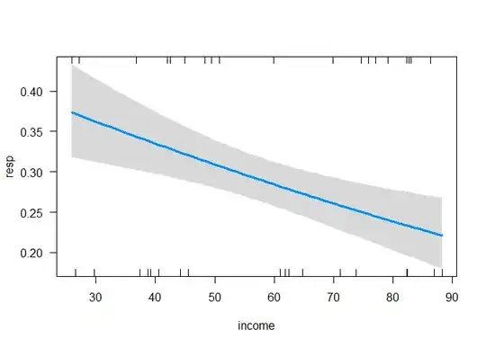
# Slope, not scaled
(0.375-0.225)/(max(FoodExpenditure$income) - min(FoodExpenditure$income))
#> [1] 0.002406623
# Slope, scaled
(0.375-0.225)/((max(FoodExpenditure$income) - min(FoodExpenditure$income))/sd(FoodExpenditure$income))
#> [1] 0.04796776
sessionInfo()
#> R version 4.2.0 (2022-04-22 ucrt)
#> Platform: x86_64-w64-mingw32/x64 (64-bit)
#> Running under: Windows 10 x64 (build 22000)
#>
#> Matrix products: default
#>
#> locale:
#> [1] LC_COLLATE=Spanish_Spain.utf8  LC_CTYPE=Spanish_Spain.utf8

#> [3] LC_MONETARY=Spanish_Spain.utf8 LC_NUMERIC=C

#> [5] LC_TIME=Spanish_Spain.utf8

#>
#> attached base packages:
#> [1] stats     graphics  grDevices utils     datasets  methods   base

#>
#> other attached packages:
#>  [1] visreg_2.7.0          forcats_0.5.1         stringr_1.5.0

#>  [4] dplyr_1.1.2           purrr_1.0.1           readr_2.1.2

#>  [7] tidyr_1.3.0           tibble_3.2.1          ggplot2_3.4.0

#> [10] tidyverse_1.3.1       glmmTMB_1.1.3         emmeans_1.8.5-9000004
#> [13] effects_4.2-1         carData_3.0-5         betareg_3.1-4

#>
#> loaded via a namespace (and not attached):
#>  [1] nlme_3.1-157        fs_1.5.2            lubridate_1.8.0

#>  [4] insight_0.19.1.3    httr_1.4.3          numDeriv_2016.8-1.1
#>  [7] tools_4.2.0         TMB_1.8.1           backports_1.4.1

#> [10] utf8_1.2.2          R6_2.5.1            DBI_1.1.2

#> [13] colorspace_2.0-3    nnet_7.3-17         withr_2.5.0

#> [16] tidyselect_1.2.0    compiler_4.2.0      cli_3.6.1

#> [19] rvest_1.0.2         xml2_1.3.3          sandwich_3.0-1

#> [22] scales_1.2.0        lmtest_0.9-40       mvtnorm_1.1-3

#> [25] digest_0.6.29       minqa_1.2.4         rmarkdown_2.14

#> [28] pkgconfig_2.0.3     htmltools_0.5.2     lme4_1.1-29

#> [31] dbplyr_2.1.1        fastmap_1.1.0       highr_0.9

#> [34] rlang_1.1.1         readxl_1.4.0        rstudioapi_0.13

#> [37] generics_0.1.2      zoo_1.8-10          jsonlite_1.8.0

#> [40] magrittr_2.0.3      modeltools_0.2-23   Formula_1.2-4

#> [43] Matrix_1.4-1        Rcpp_1.0.10         munsell_0.5.0

#> [46] fansi_1.0.3         lifecycle_1.0.3     stringi_1.7.6

#> [49] multcomp_1.4-19     yaml_2.3.5          MASS_7.3-57

#> [52] flexmix_2.3-17      grid_4.2.0          crayon_1.5.1

#> [55] lattice_0.20-45     haven_2.5.0         splines_4.2.0

#> [58] hms_1.1.1           knitr_1.39          pillar_1.9.0

#> [61] boot_1.3-28         estimability_1.4.1  codetools_0.2-18

#> [64] stats4_4.2.0        reprex_2.0.2        glue_1.6.2

#> [67] evaluate_0.15       mitools_2.4         modelr_0.1.8

#> [70] vctrs_0.6.3         nloptr_2.0.1        tzdb_0.3.0

#> [73] cellranger_1.1.0    gtable_0.3.0        assertthat_0.2.1

#> [76] xfun_0.31           xtable_1.8-4        broom_0.8.0

#> [79] survey_4.1-1        coda_0.19-4         survival_3.3-1

#> [82] TH.data_1.1-1       ellipsis_0.3.2
Created on 2023-08-01 with reprex v2.0.2