PCA to reconstruct Binary Data

Question

I'm working with binary 3D matrices. I calculate their PCA (or REOF or SVD) and as a test I would like to reconstruct these matrices from the PCA results. However I realized that because I only keep the first 10 modes of my PCA, the reconstruction ends up giving me floats between 0 and 1 rather than binary numbers.

Can a PCA reconstruction (see this question) with only the first principal components return binary numbers ? (binary in -> binary out)

Answer 1

As you mention, you can always round the output of your floating point PCA/SVD to 0/1, and that may work well enough for your purpose. But, there are other options which are tuned to the binary case and may be able to do more with fewer components (if your data has rank higher than the rank you truncate the principal subspace to).

First, since this is stats overflow, there are probabilistic options. Standard principal components analysis is derived under the assumption that the data has a multivariate normal distribution. In other words, the answer to "which low-dimensional subspace contains the most variance?" has a nice answer in the Gaussian case. Still, for non-Gaussian data (like binary data, typically modeled with the Bernoulli distribution), similar questions can be asked and answered, and these may be more appropriate for your context. For instance, you could consider looking into logistic PCA -- its relation to PCA is something like the relationship between logistic regression and the usual (Gaussian) linear regression. A. Landgraf's R package of this name may be of interest, and that website points to some nice related literature. As in logistic regression, there are lots of related models which could be of interest. For instance, although Poisson NMF models nonnegative integer data, it is also sometimes used on binary count data (although its reconstructions may not be binary).

And second, there is lots of literature about low-rank Boolean matrix factorizations -- this webpage has many references and a tutorial. Googling this term and your programming language of choice should turn up useful implementations of standard algorithms. For instance, the Nimfa package in Python includes some.

Answer 2

The reconstructed dataset using a subset of principal components is an orthogonal projection: a mathematical generalization of the process of rendering a 3D scene as an image.

This famous Escher print projects a regular array of shapes into fewer dimensions. The locations of the shapes in the paper is no longer regular (it is not a lattice).

Binary data in $n$ dimensions, whose values are limited to $0$ and $1,$ are necessarily located on the integer lattice (of vectors with integral coordinates). But when projected, even into a space of just one dimension less (as in the Escher print), they will not necessarily appear lattice-like. Here, for instance, is the projection of 16 binary vectors in $32$ dimensions onto the space spanned by their first two principal components:

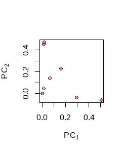
(There is some overlap in the projections, evidenced by the stronger coloration in the overlapping points, yielding only 8 distinct points.)

It therefore is unrealistic to hope either that such a "partial reconstruction" will have all binary coordinates (which would cause all the points to fall on the integer lattice) or even that rounded versions would correctly reproduce the original data.

To demonstrate this, here are the original dataset, its reconstruction based on the top five principal components, and the rounded version of that reconstruction. All are plotted as images in which each column represents a vector.

(This PCA centered all the columns but did not rescale them.) This reconstruction accounts for 87% of the variance. All the variance is accounted for by the top seven PCs, indicating this reconstruction is a projection from a space that is inherently of seven dimensions into a space of five dimensions.

You can see that many of the reconstructed coordinates are close to $0$ (lightest color) or $1$ (darkest color), but not all are. At the right, you will notice the rounded reconstruction looks substantially like the original, but not quite. About 1.2% of the coordinates flipped from $0$ to $1$ and another 2.0% of them flipped from $1$ to $0.$

---

Here, to show the details of the calculations, is the R code used to generate this example.

#
# Generate binary data.
#
set.seed(17)
p <- 16   # Number of observations
n <- 32   # Dimension of the vectors (cannot be less than `p`)
kmax <- 3 # Roughly, determines the rank of the matrix
A <- matrix(sample(0:1, p * kmax, replace = TRUE), ncol = p)
X <- (matrix(sample(0:1, n * kmax, replace = TRUE), n) %*% A) %% 2
#
# Perform PCA.
#
obj <- princomp(X)
screeplot(obj)      # Charts contributions from the highest PCs
with(obj, signif(cumsum(sdev^2)[1:10] / sum(sdev^2), 3)) # Their contributions
#
# Reconstruct the data from a specified number of PCs.
#
k <- 5 # PCs used for reconstruction
X. <- with(obj, 
           t(zapsmall(loadings[, 1:k, drop = FALSE] %*% t(scores)[1:k, , drop = FALSE] 
                      + center)))
#
# Display `X.`, `X`, and its rounded version as images.
#
par(mfrow = c(1,3))
i <- list(Reconstructed = X., Original = X, Rounded = round(X.))
for (s in names(i)) {
  image(i[[s]], bty = "n", xaxt = "n", yaxt = "n", main = s)
}
par(mfrow = c(1,1))
#
# Evaluate the differences between the original data and the rounded reconstruction.
#
table(X - round(X.)) / length(X)
with(obj, plot(loadings[, 1:2], pch = 21, bg = hsv(0.02, 1, 1, 0.3), 
               xlab = expression(PC[1]), ylab = expression(PC[2])))