How to fix this plot of histogram and pdf in R?

Question

I am studying statistics and am working with R for the first time. I have some data that I am trying to represent it graphically. I have plotted a histogram and am trying to model it with gamma distribution. I have calculated the coefficients $\lambda$ and $n$ of this gamma distribution. I defined gamma_pdf as

gamma_pdf <- function(x, lambda, n) {
  area*lambda^(n)*x^(n - 1) * exp(-lambda * x) / gamma(n)
}

I have then plotted this histogram and the pdf of this gamma distribution (scaled by the area of the histogram) and gotten the following image.

I did this using ggplot with the following code:

ggplot(data, aes(x = cas)) +
geom_histogram() +
stat_function(fun = gamma_pdf, args = list(lambda = lambda, n = n), color = "red",linewidth = 1)

Now I am trying to transform (only) the x-scale logarithmically (with base 10). Just applying function scale_x_log10() doesn't work, as it yields:

I believe I have to apply the transformation formula for the random variable $Y = \log_{10} X$. Since $$ f_X(x) = \frac{\lambda^a}{\Gamma(a)} x^{a-1} e^{- \lambda x}, $$ we get that $$ f_Y(y) = 10^y \ln(10) \frac{\lambda^a}{\Gamma(a)}10^{y(a-1)} e^{- \lambda 10^y}. $$

So I defined

log_gamma_pdf <- function(x, lambda, n) {
  newarea*10^(x)*log(10) * lambda^(n) * 10^(x*(n-1)) * exp(-lambda*10^(x)) / gamma(n)
}

and plotted the following image,

using the following code

ggplot(data, aes(x = cas)) +
  geom_histogram() +
  stat_function(fun = log_gamma_pdf, args = list(lambda = lambda, n = n), color = "red",linewidth = 1)+
  scale_x_log10()

The shape appears to be better, but something still doesn't seem to go right. I have spent the entire day playing with this, but I have no idea what I'm doing wrong. Does anyone have any advice?

---

Edit: I came to this problem by trying to solve last year's exam problems. It specifically asks to transform the x-scale logarithmically and comment if this distribution is consistent with Poisson model (exponential distribution).

I am almost certain that the graph should fit nicely, because a friend who was taking this exam last year told me that he got the 2nd graph in my question, and stated that it did not seem consistent, but was then told by the professor that had he transformed the plot correctly, he should get that it was consistent.

Also, how could the original plot seem fully consistent, but when I transform it logarithmically, it seems completely off?

Answer 1

scale_x_log10 does not transform the x-variable but only the scale of the x-axis. We can see that if we plot $f(x) = x$ with it and the result looks like the graph of $10^x$:

ggplot() + 
  stat_function(fun = function(x){x}, color = "red",linewidth = 1) +
  scale_x_log10()

Now if you use geom_histogram with scale_x_log10 it does something interesting and keeps the graphical width of all the bins the same, which of means that the real width of the bins grows exponentially with every centimeter across the x-axis, but since the true $x$ values are maintained, the used binwidth is proportional to $x$, with a factor of $\log(10)$.

library(tidyverse)
n <- 10000
bw <- 0.1
# I used Rs internal Gamma-distribution which has a slightly different parametriaztion see help("rgamma")
df <- data.frame(x = rgamma(n, shape = 4, scale = 2))
gamma_pdf <- function(x){
  dgamma(x, shape = 4, scale = 2) * bw * n
}
untransformed
ggplot(df, aes(x = x)) +
  geom_histogram(binwidth = bw) +
  stat_function(fun = gamma_pdf, color = "red",linewidth = 1)
log10 fail
ggplot(df, aes(x = x))+ 
  stat_function(fun = function(x){x}, color = "red",linewidth = 1) +
  scale_x_log10()
correct function in blue
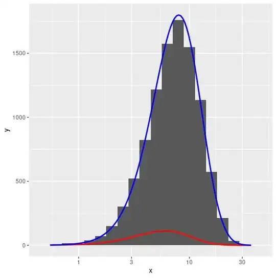
ggplot(df, aes(x = x)) +
  geom_histogram(binwidth = bw) +
  stat_function(fun = gamma_pdf, color = "red",linewidth = 1) +
  stat_function(fun = function(x){gamma_pdf(x) * x * log(10)}, color = "blue",linewidth = 1) +
  scale_x_log10()

Of course if you actually transform and make a plot $\log_{10}(x)$ then you need the full transformed pdf:

ggplot(df, aes(x = log10(x))) +
  geom_histogram(binwidth = bw) +
  stat_function(fun = gamma_pdf, color = "red",linewidth = 1) +
  stat_function(fun = function(x){gamma_pdf(x) * x * log(10)}, color = "blue",linewidth = 1) +
  stat_function(fun = function(x){gamma_pdf(10^x) * 10^x * log(10)}, color = "green",linewidth = 1) 

If you look at the formulas you can see that they are almost the same, just replace $10^x$ in the transformed PDF with $x$.