First of all, because $u$ and $d$ are parameters (constants), it's not helpful to view them as random variables. Thus, you aren't asking about a conditional probability: you want to know how to find the distribution of $Z = X/Y.$
The method I outlined in an answer to your previous question applies directly. Here I give a more concrete answer, including working code, to illustrate how this method automatically copes with the annoying details. The overall idea is to express any uniform distribution on an interval as a mixture of uniform distributions on intervals anchored at zero. This is convenient because the numbers in such intervals are all of the same sign: all non-negative or all non-positive.
The ratio of two iid standard Uniform variables
I will describe the reasoning in backwards order, beginning with the ultimate simplification: what is the distribution of the ratio of independent uniformly distributed variables on the unit interval $[0,1]$? This can be found with a simple symmetry argument -- albeit a fairly sophisticated one -- as detailed at https://stats.stackexchange.com/a/185709/919. If we call the variables $U$ and $V,$ then it is evident that $X = U/V$ and $1/X = V/U$ have the same distribution supported on the non-negative numbers. Therefore, writing the density of $X$ with respect to $\mathrm dx$ as $f_X,$ the density with respect to $\mathrm dx/x$ is $xf_X(x),$ whence the foregoing symmetry implies
$$xf_X\left(x\right) \frac{\mathrm d x}{x} = \frac{1}{x}f_X\left(\frac{1}{x}\right)\frac{\mathrm d x}{x} $$
for all $x \gt 0,$ which (by very simple algebra) is equivalent to
$$f_X(x) = \frac{1}{x^2}f_X\left(\frac{1}{x}\right).$$
In various ways (e.g., by considering $\log X$) we can discover that $f_X$ is constant on $[0,1],$ where (because this must comprise half the total probability) it equals $1/2.$ Consequently $f_X(x) = 1/(2x^2)$ for $x\ge 1.$ Let's call this the "standard uniform ratio distribution."
In the R code below this is implemented in the function pur0 ("pur" = Probability of Uniform Ratio) with the line
ifelse(x <= 0, 0, ifelse(x <= 1, 1/2, 1/(2*x^2))
which explicitly handles any negative arguments, too.
The ratio of two independent non-negative zero-anchored uniform variables.
By "zero-anchored" I mean a variable defined on an interval with $0$ as an endpoint. As a matter of notation, let "Uniform$(a,b)$" name a uniform distribution on an interval with endpoints $a$ and $b,$ no matter whether $a\le b$ or $b\le a.$
When $U \sim$ Uniform $(0,a)$ and, independently, $V \sim$ Uniform $(0,b),$ then simply changing the units of measurement of $U$ and $V$ shows that
$$(U/a)/(V/b) = \frac{b}{a}\frac{U}{V} = \frac{b}{a}X$$
has the standard uniform ratio distribution. This is implemented in the line of code
C <- abs(b / a); x <- C * x
Decomposing a Uniform distribution into a mixture
This is the mixture technique: for any numbers $a\ne b,$ the Uniform$(a,b)$ distribution is a mixture of the Uniform$(\min(a,b),0)$ and Uniform$(\max(a,b),0)$ distributions with weights
$$p = \frac{-\min(a, b)}{|b-a|};\quad q = 1-p,$$
respectively. For example, with $a=-1$ and $b=2,$ this breaks the Uniform distribution on the interval $[-1,2]$ (where its density is constantly $1/3$) into a mixture of a uniform distribution on $[-1,0]$ with weight $p=1/3$ and a uniform distribution on $[0,2]$ with weight $q=2/3.$ That much is obvious; but the interesting aspect is this analysis holds even when $a$ and $b$ have the same sign.
For example, the Uniform$(1,3)$ distribution has a constant density of $1/2$ on the interval $[1,3].$ The mixture decomposition expresses is as a Uniform distribution on the interval $[0,1]$ (constant density $1$) with negative weight $p = -1/2$ and a Uniform distribution on $[0,3]$ (constant density $1/3$) with weight $q = 1-p = 3/2.$ Sure enough, on $[0,1]$ the net density is $-1/2\times 1 + 3/2\times 1/3 = 0$ while on $[1,3]$ the net density is $-1/2\times 0 + 3/2\times 1/3 = 1/2,$ exactly as claimed.
The distribution functions can be found by integrating the densities. The only complication is that when the ratio $b/a$ is negative, the direction of integration is reversed, whence the distribution function $F_X$ must be replaced by its survival function $1-F_X.$ The line
if(isTRUE(a * b < 0)) 1 - pur0(-x) else pur0(x)
takes care of this nicety.
This analysis into a mixture is performed by the very simple function analyze in the R code. That function's argument xy is the pair of endpoints $(a,b)$. It returns a data structure giving the nonzero endpoints of the two zero-anchored intervals -- the "left" interval and the "right" interval -- along with with weight $p$ attached to the left interval.
The ratio of any two independent Uniform variables
Generally, when any random variable $X$ is a mixture of random variables $X_i$ with weights $\omega_i$ and and independent variable $Y$ is a mixture of random variables $Y_j$ with weights $\eta_j,$ then any function $Z = h(X,Y)$ is a mixture of the random variables $h(X_i,Y_j)$ with weights $\omega_i\eta_j.$
This claim is obvious (when the weights are positive) when you view a mixture as a two-step process. A realization of a mixture $X$ is achieved by first selecting an index $i$ with probability $\omega_i$ and then taking a realization of $X_i.$ Accordingly, a realization of $h(X,Y)$ is achieved by choosing $i$ and $j$ independently, obtaining realizations of $X_i$ and $Y_j,$ and computing $h(X_i,Y_j).$ The generalization to negative weights doesn't introduce anything new -- it merely leans on the measure theory that underlies all probability distributions, wherein distributions with negative (or even complex) values are considered.
The mixture calculation is performed by the last line of pur (which is the only line that does anything with the argument x: the rest is just preliminary analysis). This overloaded function computes either the density (type = "d") or distribution function (type = "p"), as requested.
There's no need to write this explicitly as a formula: it is now clear that
the general uniform ratio is a signed mixture of up to $2\times 2 = 4$ scaled standard uniform ratio distributions.
You only need to calculate the values of $p,$ $q,$ and $b/a$ for numerator and denominator.
Illustration
To illustrate, consider four possible distributions for $U$ and the same four possible distributions for $V$ covering a gamut of possibilities: Uniform$(-3,-1),$ Uniform$(-1,1),$ Uniform$(0,2),$ and Uniform$(1/2, 5/2).$ For each of the 16 possible ratios I have generated a thousand random variates according to the numerator and denominator, computed their ratios, plotted the empirical distribution of those ratios (in black) and superimpose the theoretical distribution function (in red).

The agreement between theory and simulation is excellent. This tableau gives us a sense of what the possible distribution functions might look like.
Repeating the procedure (this time with 40 thousand random values per plot to provide more detail) and drawing the histograms on which the computed density functions are plotted gives this illustration:
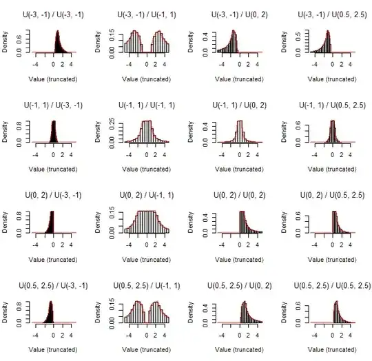
Again agreement between simulation and calculation is excellent. (Some of the distributions have extremely long tails -- division by values near zero will do that -- so to make these plots I have truncated all results to the range $[-5,5]$ and plotted the truncated densities.)
Close study of these plots will be rewarding insofar as it can help you develop an intuition for the operations carried out during this analysis, including scaling, shifting, and taking ratios of distributions.
R code
Here is a full implementation of the general Uniform Ratio distribution functions pur and density functions dur. Their parameters are ab (the endpoints of the numerator) and cd (the endpoints of the denominator).
analyze <- function(xy = c(0, 1)) {
  obj <- list(Left = min(xy), Right = max(xy))
  dr <- abs(diff(xy))
  obj$p <- ifelse(dr <= 0, 0, -(obj$Left) / dr)
  obj
}
pur. <- function(x, ab, cd, type = c("p", "d")) {
  # Case of U[0,1] divided by U[0,1].
  if (isTRUE(type == "p")) {
    pur0 <- function(x) ifelse(x <= 0, 0, ifelse(x <= 1, x/2, 1 - 1/(2*x)))
  } else {
    pur0 <- function(x) ifelse(x <= 0, 0, ifelse(x <= 1, 1/2, 1/(2*x^2)))
  }
  # Case of U[0,a] divided by U[0,b].
  pur1 <- function(x, a, b) {
    if(isTRUE(a == 0)) {sign(x) # Needed to avoid division by zero
    } else {
      C <- abs(b / a); x <- C * x
      if (isTRUE(type == "p")) {
        if(isTRUE(a * b < 0)) 1 - pur0(-x) else pur0(x)
      } else {
        pur0(x * sign(a * b)) * C
      }
    }
  }
  # Mixture decomposition.
  AB <- analyze(ab); CD <- analyze(cd)
  AB$p * CD$p * pur1(x, AB$Left, CD$Left) +
    (1 - AB$p) * CD$p * pur1(x, AB$Right, CD$Left) +
    AB$p * (1 - CD$p) * pur1(x, AB$Left, CD$Right) +
    (1 - AB$p) * (1 - CD$p) * pur1(x, AB$Right, CD$Right)
}
pur <- function(x, ab = c(0, 1), cd = c(0, 1)) pur.(x, ab, cd, "p")
dur <- function(x, ab = c(0, 1), cd = c(0, 1)) pur.(x, ab, cd, "d")


