First, let's recall the necessary formulas (with a slight change in notation with respect to the post). As a bonus to your query, I'm considering also prediction intervals. Let $\mu_f = \beta_1 + \beta_2 x_f$ be the conditional average of $Y$ at $X = x_f$. An estimator for this is $\hat Y_f = \hat \beta_1 + \hat \beta_2 x_f$. Thus $\hat Y_f = \bar Y + \hat\beta_2(x_f-\bar x)$.
Under the linear regression assumptions, we have the pivot
$$
\frac{\hat Y_f-\mu_f}{S\sqrt{\frac{1}{n}+\frac{(x_f-\bar x)^2}{\sum_{i=1}^n(x_i-\bar x)^2}}}\sim t_{n-2},\tag{*}
$$
where $S^2 = \frac{1}{n-2}\sum (Y_i-\hat\beta_0-\hat\beta_1x_i)^2$ is the corrected residual variance.
From (*), we can build a confidence interval of $1-\alpha$ for $\mu_f$ as
$$\left[\hat Y_f \pm t_{n-2, 1-\alpha/2}S\sqrt{\frac{1}{n}+\frac{(x_f-\bar x)^2}{\sum_{i=1}^n(x_i-\bar x)^2}}\right].$$
On the other hand, the prediction interval for $\mu_f$ is given by
$$\left[\hat Y_f \pm t_{n-2, 1-\alpha/2}S\sqrt{1+\frac{1}{n}+\frac{(x_f-\bar x)^2}{\sum_{i=1}^n(x_i-\bar x)^2}}\right].$$
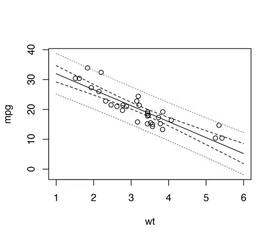
The following R code illustrates how to compute all these quantities and combine them to obtain the desired plot. Instead of computing the necessary quantities "by hand" using the above expression for the confidence/prediction interval, I'll show how to do it by taking advantage of suitable R functions, e.g. predict.
# fit the model
my_lm <- lm(mpg~wt, data = mtcars)
generate some new data
new_data = data.frame(wt = seq(1,6,len=length(mtcars$wt)))
compute the confidence interval for the regression line
ci <- predict(my_lm, newdata = new_data, interval = "confidence")
compute the prediction interval
ci_pred <- predict(my_lm, newdata = new_data, interval = "prediction")
combine everything
plot(mpg~wt, data = mtcars, xlim = range(new_data$wt),
     ylim =range(ci_pred))
matlines(new_data$wt, ci, lty = c(1,2,2), col=c(1,1,1))
matlines(new_data$wt, ci_pred[,-1], lty = c(3,3), col=c(2,2))