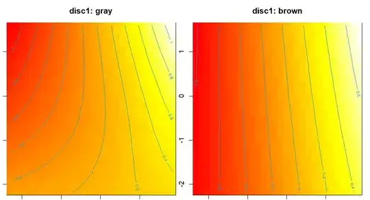
GAM: covariate specific fits do not appear to match approximate significance of smooth terms

Question

I have fit a GAM with two continuous independent variables and one discrete covariate with two levels ("gray" and "brown"). All variables are scaled and the model runs fine:

mod3 = gam(cont1 ~ disc1 * cont2 * cont3 + 
             s(cont2, cont3, by=disc1, k=4),
           data=data_so)
summary(mod3)
Family: gaussian 
Link function: identity
Formula:
cont1 ~ disc1 * cont2 * cont3 + s(cont2, cont3, by = disc1, k = 4)
Parametric coefficients:
                           Estimate   Std. Error  t value   Pr(>|t|)
(Intercept)             0.015009690  0.038191859  0.39301 0.69440639
disc1brown             -0.032717084  0.066537035 -0.49171 0.62304187
cont2                   0.212856916  0.018793283 11.32622 < 2.22e-16
cont3                   0.005457858  0.019394264  0.28142 0.77845557
disc1brown:cont2        0.061748331  0.021911015  2.81814 0.00493549
disc1brown:cont3        0.016191669  0.027321828  0.59263 0.55357838
cont2:cont3             0.118947202  0.035662553  3.33535 0.00088654
disc1brown:cont2:cont3 -0.098224982  0.071036399 -1.38274 0.16708507
Approximate significance of smooth terms:
                                edf    Ref.df       F   p-value
s(cont2,cont3):disc1gray  1.8362810 2.0676743 1.08907 0.1846056
s(cont2,cont3):disc1brown 0.7998747 0.7998747 9.65092 0.0055757
Rank: 10/14
R-sq.(adj) =  0.128   Deviance explained = 13.5%
GCV = 0.88013  Scale est. = 0.87182   n = 914

However, the approximate significance of each smooth term does not match my a priori expectation. More importantly, it also doesn't match the visualized model fit, by which "gray" should be non-linear, and "brown" somewhat linear:

vis.gam(mod3, view=c("cont2","cont3"), plot.type="contour", 
        cond=list(disc1="gray"), main="disc1: gray")
vis.gam(mod3, view=c("cont2","cont3"), plot.type="contour", 
        cond=list(disc1="brown"), main="disc1: brown")

If I run the model only with either class, it appears to match the figure (high F/low P value for approx. sign. of smooth term for "gray, and the opposite for the "brown" model:

> mod3a = gam(cont1 ~ cont2 * cont3 + 
+               s(cont2, cont3, k=4),
+             data=data_so[disc1=="gray"])
> summary(mod3a)
Family: gaussian 
Link function: identity
Formula:
cont1 ~ cont2 * cont3 + s(cont2, cont3, k = 4)
Parametric coefficients:
                Estimate   Std. Error  t value   Pr(>|t|)
(Intercept)  0.021064013  0.038786204  0.54308  0.5872749
cont2        0.175710375  0.019469841  9.02475 < 2.22e-16
cont3       -0.003258934  0.019493737 -0.16718  0.8672855
cont2:cont3  0.118727033  0.036447026  3.25752  0.0011869
Approximate significance of smooth terms:
                    edf   Ref.df        F    p-value
s(cont2,cont3) 1.590295 1.828967 34.76433 < 2.22e-16
Rank: 5/7
R-sq.(adj) =  0.127   Deviance explained = 13.2%
GCV = 0.91631  Scale est. = 0.90938   n = 609
> mod3b = gam(cont1 ~ cont2 * cont3 +

          s(cont2, cont3, k=4),


        data=data_so[disc1==&quot;brown&quot;])



> summary(mod3b)
Family: gaussian 
Link function: identity
Formula:
cont1 ~ cont2 * cont3 + s(cont2, cont3, k = 4)
Parametric coefficients:
               Estimate  Std. Error  t value          Pr(>|t|)
(Intercept) -0.01997134  0.05075102 -0.39352           0.69422
cont2        0.17893076  0.02588782  6.91177 0.000000000028642
cont3        0.01326603  0.02519297  0.52658           0.59888
cont2:cont3  0.02072222  0.05873067  0.35283           0.72446
Approximate significance of smooth terms:
                    edf   Ref.df       F p-value
s(cont2,cont3) 1.075582 1.075582 2.71988 0.06871
Rank: 5/7
R-sq.(adj) =  0.133   Deviance explained = 14.2%
GCV = 0.80732  Scale est. = 0.79673   n = 305

What is going on here? Might be related: Why do gam predictions not match gam smooth?

Two comments: 1) There usually isn't a need to use standardized scaling for GAM(M)s and makes the model less interpretable 2) You should really consider using something like method=REML, as the default GCV is not recommended. — Shawn Hemelstrand, Mar 13 '23 at 10:44
ad 1) I standardized the data because they are on vastly different scales (how does mgcv::gam deal with that?), and because I use the same standardized data in analyses where I have to standardize. ad 2) you mean always or just in this context? — mluerig, Mar 13 '23 at 10:52
If by "the visualized model fit" you mean the plots of the smoothers then I don't understand the question. p-values take into account uncertainty but the plots do not depict uncertainty. Also, I don't understand why you include both linear effects for the continuous predictors and a smoother. Why not just include a tensor product smoother? — Roland, Mar 13 '23 at 11:22
@mluerig Roland alludes to what I already was going to say. Tensor products include the raw data without any need for standardization. It's one of the massive benefits of a GAM over a GLM because there is no need to standardize variables for interactions. As for GCV, it almost always undersmooths. Read Page 8 of https://www.frontiersin.org/article/10.3389/fevo.2018.00149/full — Shawn Hemelstrand, Mar 13 '23 at 11:51

Shawn Hemelstrand · Accepted Answer · 2023-03-13T15:34:56.357

So there are a number of issues I have to address here. First off, you should almost never use GCV, as it typically undersmooths and creates overly "wiggly" lines in your GAM (Simpson, 2018). Second, if you use a tensor product term, there is no need to standardize your variables in the model (see Baayen et al., 2017 and Pedersen et al., 2019 for more info on these). I express why standardization is problematic from a practical view in this answer.

But by far the biggest issue I see in your model is you have actually modeled most of your variables as parametric coefficients, which means they have no estimated curvilinearity in your regression. In order to estimate main effects as well as the interaction of each variable, you should give each their own spline. I'm assuming what you actually wanted was something like this:

mod3 <- gam(cont1 
           ~ disc1
           + s(cont2) 
           + s(cont3)
           + ti(cont2, 
                cont3,
                by=disc1, 
                k=c(4,4),
           data = data_so,
           method = "REML")

An example of what this is doing is shown here in Baayen et al., 2017 (here they use ti for the main effect splines, but s for main effects is functionally equivalent):

This may be partially why your interactions don't match expectation. So you should revise your model to have proper spline terms first, then try to understand what is going on thereafter.

Citations

Baayen, H., Vasishth, S., Kliegl, R., & Bates, D. (2017). The cave of shadows: Addressing the human factor with generalized additive mixed models. Journal of Memory and Language, 94, 206–234. https://doi.org/10.1016/j.jml.2016.11.006
Pedersen, E. J., Miller, D. L., Simpson, G. L., & Ross, N. (2019). Hierarchical generalized additive models in ecology: An introduction with mgcv. PeerJ, 7, e6876. https://doi.org/10.7717/peerj.6876
Simpson, G. L. (2018). Modelling palaeoecological time series using generalised additive models. Frontiers in Ecology and Evolution, 6(149), 1–21. https://doi.org/10.3389/fevo.2018.00149

yupp that "*" was a problem - thanks for fixing. also, you are missing a ")" — mluerig, Mar 13 '23 at 15:53
re. GCV: I have used it in the past, and simply constrained the knots to lowest number possible - doesn't that partially take care of overly wiggly smooths? — mluerig, Mar 13 '23 at 15:54
There are other issues with it outlined here https://stats.stackexchange.com/a/581293/345611 — Shawn Hemelstrand, Mar 13 '23 at 16:02

GAM: covariate specific fits do not appear to match approximate significance of smooth terms

1 Answers1

Citations