6

$X$ and $Y$ are two non-negative continuous random variables. The moments of $X$ are $\mu_i$ while that of $Y$ are $\nu_i$.

We know that $\mu_1=\nu_1$ and $\mu_i \ge \nu_i$ for $i=2,3,\ldots$

Can one then show that $P(X>x) \ge P( Y>x)$ for $x\ge \mu_1$?

We do know that $$ \mu_i=i\int_{0}^{\infty} x^{i-1} P(X>x) dx \ge i\int_{0}^{\infty} x^{i-1} P(Y>y) dx = \nu_i$$ for all $i$.

It holds for the special case where $\nu_i=0$ for $i=2,3,\ldots$

Richard Hardy
  • 67,272
GCru
  • 235

2 Answers2

9

The conclusion does not follow. The family of distributions described at How is the kurtosis of a distribution related to the geometry of the density function? gives a counterexample. These are densities $f_{k,s}$ all of which have identical moments. If we were, then, to shift one of them by some positive amount, all its moments would (strictly) increase. Here is a plot of their distribution functions $F_{k,s}$ (evaluated numerically):

enter image description here

Clearly neither dominates the other, even though all the moments of the red distribution exceed those of the black distribution.


For those who would like to experiment with this family, here is the R code used to create these plots.

f <- function(x, k=0, s=0) {
  ifelse(x <= 0, 0, dnorm(log(x)) * (1 + s * sin(2 * k * pi * log(x))) / x)
}
ff <- Vectorize(function(x, k=0, s=0, ...) {
  integrate(\(y) f(y, k, s), 0, x, ...)$value
})
curve(ff(x), 0, 4, lwd = 2, ylim = 0:1, 
      ylab = "Probability", xlab = expression(italic(x)), cex.lab = 1.25)
curve(ff(x - 0.01, 1, 3/4), add = TRUE, lwd = 2, col = "Red")
User1865345
  • 8,202
whuber
  • 322,774
  • 3
    I missed your assumption that the first moments are equal. If we shift $Y$ by $\epsilon$ and scale it by $(1+\epsilon)^{-1},$ further analysis (relying on the values of these lognormal moments) shows all the higher moments of $Y$ are strictly less than those of $X.$ For sufficiently small $\epsilon,$ the negative result continues to hold. – whuber Nov 25 '22 at 17:15
  • 1
    Thank you @whuber for such an instructive counter example! – GCru Nov 25 '22 at 17:46
7

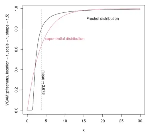
The higher moments say relatively little about the behaviour of the distribution at small values. The tails have a lot of influence on a distribution.

You can see this in particular with distributions that have infinite higher moments.

For example compare a Frechet distribution with location = 1, scale = 1 and shape = 1.5 (this has finite mean but infinite variance) to an exponential distribution with equal mean.

example with Frechet versus exponential