When does the standard errors of OLS estimates decreases when we have more explanatory variables?

Question

So far my understanding is that standard errors of $\hat\beta_j$ increase when we have more independent variables in the regression model because variation among those independent variables will increase ($\rightarrow R^2_j \uparrow$). But I saw the opposite thing happened when I add more explanatory variables in the RHS of the simple difference-in-differences model:

$$y_t=\beta_0+\delta_0x_1+\beta_1 x_2+\delta_1x_1x_2+u $$

I can't understand how this could be possible?

Answer 1

This can happen for a few reasons. One scenario is as follows:

Consider a model

$$ y = \beta_0 + \beta_1x + \beta_2 w + \beta_3 z + \epsilon $$

Suppose that the covariate $x$ is randomly assigned to units in the population. Hence $x$ is uncorrelated with any other variables $w, z$ considered for adjustment by construction.

If $w$ and $z$ can explain variation in $y$, then the standard error for $\beta_1$ (the coefficient for the randomly allocated $x$) can decrease as compared to the model $y = \beta_0 + \beta_1 x$.

This happens because the estimate of the residual variation $\sigma$ will decreases (due to variation in from $w$ and $z$ explaining away variation in $y$) and the covariance for beta is a function of $\sigma$.

We can very easily see this if we just simulate the model

set.seed(0)
N <- 1000
x <- rbinom(N, 1, 0.5)
w <- rnorm(N)
z <- rnorm(N)
y <- 1 + x + w + z + rnorm(N, 0, 0.5)
model without w, z
vcov(lm(y~x))['x', 'x']
#> [1] 0.009220088
Look at the residual variance, nearly thrice as big as it should be
sd(resid(lm(y~x)))
#> [1] 1.516374
Model with w, x
vcov(lm(y~x + w + z))['x', 'x']
#> [1] 0.0008677971
Look at the residual variance, much closer to the true value
sd(resid(lm(y~x+w+z)))
#> [1] 0.4643699

^{Created on 2022-11-24 by the reprex package (v2.0.1)}

Answer 2

There are competing by factors. You’ve identified the variance inflation factor (VIF), and you are right that adding more variables can increase the VIF. However, another factor is how large the residual variance is. After all, a major factor in the standard of your parameter estimates is the residual variance.

Consequently, the standard error of your parameter estimates decreases when the decrease in residual variance overwhelms whatever increases to VIF occur due to adding in new features.

Answer 3

Let's do the math.

Consider zero-mean variables, and the following two regressions:

$$y = \beta x + u$$ $$y = \gamma x + \delta z + v$$

In the first model, we have $${\rm Var}(\hat \beta) = \frac{\hat \sigma^2_u}{\sum{x^2}} \tag{1}$$

In the second model we have

\begin{align}{\rm V}(\hat \gamma, \hat \delta) &= \hat \sigma^2_u \left[\begin{matrix} \sum x^2 & \sum xz\\ \sum xz & \sum z^2\end{matrix}\right]^{-1} \\ \\ &= \frac{\hat \sigma^2_u}{\left(\sum x^2\right)\left(\sum z^2\right) - \left(\sum xz\right)^2}\left[\begin{matrix} \sum z^2 & -\sum xz\\ -\sum xz & \sum x^2\end{matrix}\right]. \end{align}

The "strange" behavior is when \begin{align} {\rm Var}(\hat \gamma) < {\rm Var}(\hat \beta) &\implies \frac{\hat \sigma^2_v\sum z^2}{\left(\sum x^2\right)\left(\sum z^2\right) - \left(\sum xz\right)^2}< \frac{\hat \sigma^2_u}{\sum{x^2}}\\ \\ &\implies \frac{\hat \sigma^2_v}{\hat \sigma^2_u} < \frac{\left(\sum x^2\right)\left(\sum z^2\right) - \left(\sum xz\right)^2}{\left(\sum x^2\right)\left(\sum z^2\right)}\\ &\implies \frac{\hat \sigma^2_v}{\hat \sigma^2_u} < 1- \hat \rho^2_{xz}. \end{align}

We know that the estimated error variance in the augmented model, $\hat \sigma_v^2$ will be smaller than the corresponding estimate in the short model $\hat \sigma_u^2$.

So if this reduction is bigger (as a percentage and in absolute terms) than the squared correlation of the two variables, we will observe reduced standard error in the larger model.

If the squared correlation is zero ($x$ and $z$ are uncorrelated), then we will certainly get smaller standard deviation of the coefficient of $x$ in the augmented model.

But wait, didn't we just add a lot of independent variation in the model (but presumably related to the dependent variable)? Indeed we did, and this is exactly why "certainty" increased. It is variation that explains.

Answer 4

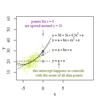
This happens mostly with misspecified models that have large residuals because of a misspecified model and that can be reduced by adding more variables.

As simple illustration can be made with simple linear regression.

• The linear model fit $x=a+bx$ in the upper left corner is more precise in the estimate at x=0. The estimate for the standard error is small because the residuals are small.
• The model that uses only an intercept $x=a$ indicates a larger error. The reason is that the residuals are much larger. With the linear model fit these residuals are a lot reduced.
• The lower right image: to our eye it seems weird that the model $y=a$ is doing bad but that is because our brain sees the linear relationship and we imagine a line going through 0. The model doesn't see this and includes no information about $x$. For the model it looks like the $x$ data are scrambled.

Another illustration that shows it dramatically is from Why is the intercept in multiple regression changing when including/excluding regressors?

A smaller model can have bias which increases the error.