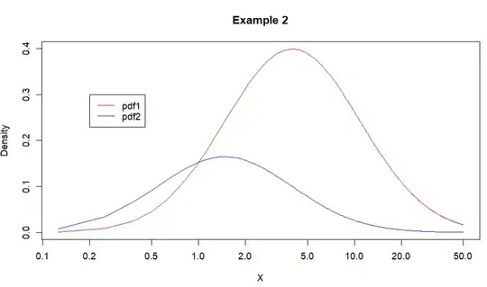
I am having trouble understanding when PDFs of transformed variables need to be modified (i.e., take derivative) for proper plotting. I've looked at Intuitive explanation for density of transformed variable? and several other resources. Here, I will give 3 examples of different x-axes, and I hope someone can help me understand which PDF is correct for each axis.
Given:
$\ln(X) \sim \mathcal{N}(\mu,\,\sigma^{2})\,$
And use R to generate plots, where pdf1 is unadjusted and pdf2 is transformed by the derivative of $ln(X)$ (i.e., $\frac{1}{X}$):
X = seq(0, 50, length.out = 400)
pdf1 = dnorm(log(X), mean=log(4), sd=1)
pdf2 = dnorm(log(X), mean=log(4), sd=1) * 1/X
Example 1 using linear X units and axis, which is correct?
plot(x=X, y=pdf1, type="l", col="red", ylab="Density")
lines(x=X, y=pdf2, type="l", col="blue")
title(main="Example 1")
legend(40, 0.3, legend=c("pdf1", "pdf2"), col=c("red", "blue"), lty=1)
Example 2 using linear X units with log axis, which is correct?
plot(x=X, y=pdf1, type="l", col="red", ylab="Density", log="x")
lines(x=X, y=pdf2, type="l", col="blue")
title(main="Example 2")
legend(0.2, 0.3, legend=c("pdf1", "pdf2"), col=c("red", "blue"), lty=1)
Example 3 using log X units with linear axis, which is correct?
plot(x=log(X), y=pdf1, type="l", col="red", ylab="Density")
lines(x=log(X), y=pdf2, type="l", col="blue")
title(main="Example 3")
legend(-2, 0.3, legend=c("pdf1", "pdf2"), col=c("red", "blue"), lty=1)


