Compute likelihood associated with indicator function and MLE $\lambda$

Question

Let $Y_1, . . . , Y_n$ be a random sample from a Poisson distribution with parameter $\lambda > 0$. One observes only $W_i = I_{Y_i>0}$ (indicator function). Compute the likelihood associated with the sample $(W_1, \ldots, W_n)$ and the MLE in $\lambda$.

I attempted this problem, but have not obtained results that seem likely. Well, Poisson is always greater than zero for parameter greater than 0, so the likelihood function would only be 1. Am I missing something?

Answer 1

The likelihood for a sample of size $n$ will be $$ \begin{eqnarray*} L(\lambda) &=&\prod_{i=1}^nf(W_i;\lambda)\\ &=&\prod_{i=1}^n\{I(W_i=0)P(Y_i=0)+I(W_i=1)P(Y_i>0)\}\\ &=&\prod_{i=1}^n\{I(W_i=0)e^{-\lambda}+I(W_i=1)(1-e^{-\lambda})\}\\ &=&e^{-n_0\lambda}(1-e^{-\lambda})^{n_1}, \end{eqnarray*} $$ where $n_0$ and $n_1$ denotes the number of zeros and ones in the sample, such that $n_0+n_1=n$.

Hence, the log-likeihood is $$ \ln L(\lambda)=n_1\ln(1-e^{-\lambda})-\lambda n_0, $$ with derivative $$ \frac{\partial \ln L(\lambda)}{\partial \lambda}=n_1\frac{e^{-\lambda}}{1-e^{-\lambda}}-n_0=\frac{n_1e^{-\lambda}-n_0(1-e^{-\lambda})}{1-e^{-\lambda}} $$ Since the denominator is positive in view of $\lambda>0$, it is enough to set the numerator to zero for the first-order condition and solve to get $$ \hat\lambda=\ln\left(\frac{n}{n_0}\right) $$

The estimator unsurprisingly will be less efficient than the full MLE (the sample mean), but also seems to be unbiased as per this little simulation.

lambda <- 2
n <- 100
mles <- function(n){
  x <- rpois(n, lambda)
  mle <- mean(x)
  n_0 <- length(x[x==0])
  mle.trunc <- log(n/n_0)
  return(c(mle, mle.trunc))
}
mle.estimates <- replicate(100000, mles(n))
plot(density(mle.estimates[1,]), lwd=2, col="lightblue")
lines(density(mle.estimates[2,]), lwd=2, col="salmon")
summary(mle.estimates[2,])
> summary(mle.estimates[2,])
   Min. 1st Qu.  Median    Mean 3rd Qu.    Max. 
  1.238   1.833   2.040   2.034   2.207   4.605

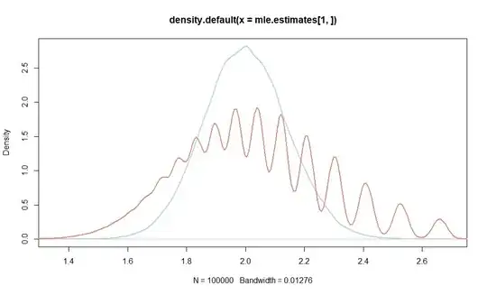
Its distribution looks a little funny though, in view of the discrete steps that $n_0$ will take for small sample sizes $n$. More concretely, $n_0\in\{0,1,\ldots,n\}$. Hence, for $n=100$ as in the example, $$ \hat\lambda\in\{\infty,4.61,3.91,\ldots,0.02,0.01, 0\}. $$ That the distribution of the estimator still looks continuous therefore also is an artefact of density. You could inspect the estimates found with, e.g., rev(sort(unique(mle.estimates[2,]))). In a simulation with 1e7 replications I got only 36 different estimates.

We may make the inefficiency of this estimator a little more formal through the asymptotic variance of the estimator via the delta method.

Since $$ \frac{n_0}{n}=\frac{1}{n}\sum_i\mathbb{I}(Y_i=0)$$ finds the proportion of zeros and estimates $$p:=P(Y_i=0)=\exp(-\lambda),$$ we have that, by properties of the binomial distribution, $$ \sqrt{n}(n_0/n-p)\to_dN(0,p(1-p)) $$ With $\log(n/n_0)=-\log(n_0/n)$, let $g(p)=-\log(p)$. Note that $g(p)=\lambda$. Then, $g'(p)=-1/p$, so that the delta method gives $$ \sqrt{n}(\log(n/n_0)-\lambda)\to_dN(0,p(1-p)/p^2) $$ Here, the asymptotic variance is $$ \frac{\exp(-\lambda)(1-\exp(-\lambda))}{\exp(-2\lambda)}=\exp(\lambda)-1 $$ Since $Var(Y_i)=\lambda$, the standard sample mean MLE has, from the central limit theorem, asymptotic variance $\lambda$, and $$ \exp(\lambda)-1>\lambda $$ for $\lambda>0$.

We observe that the variance increases in $\lambda$. This, I argue, is intuitive as the estimator only exploits whether or not $Y_i=0$, and, for $\lambda$ large, we will observe few such zeros and it will be difficult to determine which $\lambda$ is "responsible" for having produced the number of observed zeros.

Incidentally, the wobbly distribution is to a lesser extent true of the sample mean, where the integer draws from the Poisson distribution also limit the possible values of the estimator, although that effect will only be visible for even smaller $n$. For example, I found length(unique(mle.estimates[1,])) 143 different sample means in my simulation.

The following bar chart gives correct spaces between the realizations (not that it matters too much for the plot) for my draws as there are no gaps in the values actually taken vs. those that could have been taken, as per rev(log(n/0:n)) %in% sort(unique(mle.estimates[2,])):

table.estimates <- table(mle.estimates[2,!is.infinite(mle.estimates[2,])])
barplot(table.estimates, space = c(1, tail(rev(diff(sort(unique(mle.estimates[2,])))),-1)), names.arg = round(head(sort(unique(mle.estimates[2,])),-1),2))