R and Time Series Analysis; Suggestions for forecasting a series with a shock

Question

I believe that the reprex below is self-explanatory. I would like to extend a monthly time series by forecasting the next 3 data points. The series is rather volatile and it spikes during the last couple of years. By naked eye, its monthly returns fluctuate around a constant value. I am learning the ropes of time series analysis and I need something quick to implement and reasonable (possibly in R).

If it was within the tidymodels framework (see comments in the reprex), it would be ideal, but it is not crucial.

Many thanks!

library(tidyverse)
df <- structure(list(t = structure(c(2191, 2222, 2251, 2282, 2312, 
2343, 2373, 2404, 2435, 2465, 2496, 2526, 2557, 2588, 2616, 2647, 
2677, 2708, 2738, 2769, 2800, 2830, 2861, 2891, 2922, 2953, 2981, 
3012, 3042, 3073, 3103, 3134, 3165, 3195, 3226, 3256, 3287, 3318, 
3346, 3377, 3407, 3438, 3468, 3499, 3530, 3560, 3591, 3621, 3652, 
3683, 3712, 3743, 3773, 3804, 3834, 3865, 3896, 3926, 3957, 3987, 
4018, 4049, 4077, 4108, 4138, 4169, 4199, 4230, 4261, 4291, 4322, 
4352, 4383, 4414, 4442, 4473, 4503, 4534, 4564, 4595, 4626, 4656, 
4687, 4717, 4748, 4779, 4807, 4838, 4868, 4899, 4929, 4960, 4991, 
5021, 5052, 5082, 5113, 5144, 5173, 5204, 5234, 5265, 5295, 5326, 
5357, 5387, 5418, 5448, 5479, 5510, 5538, 5569, 5599, 5630, 5660, 
5691, 5722, 5752, 5783, 5813, 5844, 5875, 5903, 5934, 5964, 5995, 
6025, 6056, 6087, 6117, 6148, 6178, 6209, 6240, 6268, 6299, 6329, 
6360, 6390, 6421, 6452, 6482, 6513, 6543, 6574, 6605, 6634, 6665, 
6695, 6726, 6756, 6787, 6818, 6848, 6879, 6909, 6940, 6971, 6999, 
7030, 7060, 7091, 7121, 7152, 7183, 7213, 7244, 7274, 7305, 7336, 
7364, 7395, 7425, 7456, 7486, 7517, 7548, 7578, 7609, 7639, 7670, 
7701, 7729, 7760, 7790, 7821, 7851, 7882, 7913, 7943, 7974, 8004, 
8035, 8066, 8095, 8126, 8156, 8187, 8217, 8248, 8279, 8309, 8340, 
8370, 8401, 8432, 8460, 8491, 8521, 8552, 8582, 8613, 8644, 8674, 
8705, 8735, 8766, 8797, 8825, 8856, 8886, 8917, 8947, 8978, 9009, 
9039, 9070, 9100, 9131, 9162, 9190, 9221, 9251, 9282, 9312, 9343, 
9374, 9404, 9435, 9465, 9496, 9527, 9556, 9587, 9617, 9648, 9678, 
9709, 9740, 9770, 9801, 9831, 9862, 9893, 9921, 9952, 9982, 10013, 
10043, 10074, 10105, 10135, 10166, 10196, 10227, 10258, 10286, 
10317, 10347, 10378, 10408, 10439, 10470, 10500, 10531, 10561, 
10592, 10623, 10651, 10682, 10712, 10743, 10773, 10804, 10835, 
10865, 10896, 10926, 10957, 10988, 11017, 11048, 11078, 11109, 
11139, 11170, 11201, 11231, 11262, 11292, 11323, 11354, 11382, 
11413, 11443, 11474, 11504, 11535, 11566, 11596, 11627, 11657, 
11688, 11719, 11747, 11778, 11808, 11839, 11869, 11900, 11931, 
11961, 11992, 12022, 12053, 12084, 12112, 12143, 12173, 12204, 
12234, 12265, 12296, 12326, 12357, 12387, 12418, 12449, 12478, 
12509, 12539, 12570, 12600, 12631, 12662, 12692, 12723, 12753, 
12784, 12815, 12843, 12874, 12904, 12935, 12965, 12996, 13027, 
13057, 13088, 13118, 13149, 13180, 13208, 13239, 13269, 13300, 
13330, 13361, 13392, 13422, 13453, 13483, 13514, 13545, 13573, 
13604, 13634, 13665, 13695, 13726, 13757, 13787, 13818, 13848, 
13879, 13910, 13939, 13970, 14000, 14031, 14061, 14092, 14123, 
14153, 14184, 14214, 14245, 14276, 14304, 14335, 14365, 14396, 
14426, 14457, 14488, 14518, 14549, 14579, 14610, 14641, 14669, 
14700, 14730, 14761, 14791, 14822, 14853, 14883, 14914, 14944, 
14975, 15006, 15034, 15065, 15095, 15126, 15156, 15187, 15218, 
15248, 15279, 15309, 15340, 15371, 15400, 15431, 15461, 15492, 
15522, 15553, 15584, 15614, 15645, 15675, 15706, 15737, 15765, 
15796, 15826, 15857, 15887, 15918, 15949, 15979, 16010, 16040, 
16071, 16102, 16130, 16161, 16191, 16222, 16252, 16283, 16314, 
16344, 16375, 16405, 16436, 16467, 16495, 16526, 16556, 16587, 
16617, 16648, 16679, 16709, 16740, 16770, 16801, 16832, 16861, 
16892, 16922, 16953, 16983, 17014, 17045, 17075, 17106, 17136, 
17167, 17198, 17226, 17257, 17287, 17318, 17348, 17379, 17410, 
17440, 17471, 17501, 17532, 17563, 17591, 17622, 17652, 17683, 
17713, 17744, 17775, 17805, 17836, 17866, 17897, 17928, 17956, 
17987, 18017, 18048, 18078, 18109, 18140, 18170, 18201, 18231, 
18262, 18293, 18322, 18353, 18383, 18414, 18444, 18475, 18506, 
18536, 18567, 18597, 18628, 18659, 18687, 18718, 18748, 18779, 
18809, 18840, 18871, 18901, 18932, 18962, 18993, 19024, 19052, 
19083, 19113, 19144), class = "Date"), y1 = c(50, 50.1, 50.3, 
50.8, 50.9, 51.2, 51.4, 51.5, 51.6, 51.6, 51.5, 51.5, 51.8, 52.2, 
52.3, 52.5, 52.5, 52.5, 52.5, 52.5, 52.5, 52.5, 52.5, 52.5, 52.6, 
52.6, 52.7, 52.8, 53.2, 53.2, 53.2, 53.2, 53.2, 53.2, 53.3, 53.4, 
53.8, 54.1, 54.6, 55, 55.2, 55.4, 55.9, 56, 56.2, 56.6, 56.8, 
57.1, 57.9, 58.3, 58.8, 59.6, 59.9, 59.9, 60, 60, 60, 60.5, 61, 
61.2, 61.9, 62.3, 62.8, 63.6, 64, 64.3, 64.9, 65.3, 65.4, 66.1, 
66.3, 66.4, 67.3, 67.3, 67.3, 67.8, 68, 68.4, 68.6, 68.6, 68.6, 
69, 69, 68.8, 68.8, 68.7, 68.6, 68.8, 68.9, 69.1, 69.2, 69.5, 
69.7, 69.7, 69.9, 70, 70.4, 70.4, 70.5, 71, 71.1, 71.2, 71.3, 
71.3, 71.5, 72, 72, 72, 72.4, 72.7, 72.8, 73, 73.1, 73.1, 73.2, 
73, 73.1, 73, 72.9, 72.8, 72.7, 72.4, 72.1, 71.7, 71.4, 71.4, 
71, 70.8, 70.8, 69.8, 69.6, 69.5, 69.5, 69.3, 69.3, 69.1, 69.2, 
69.3, 69.5, 69.5, 69.5, 69.6, 69.6, 69.6, 69.6, 69.6, 69.7, 69.9, 
70.1, 70.3, 70.3, 70.4, 70.4, 70.5, 70.7, 70.9, 71.6, 71.8, 72.1, 
72.4, 72.4, 72.4, 72.4, 72.5, 72.6, 73, 72.9, 72.9, 73, 73, 73.1, 
73.5, 73.6, 73.6, 73.5, 73.9, 74.3, 74.5, 74.4, 74.1, 74.7, 74.7, 
74.5, 75.2, 75.3, 75.4, 75.9, 75.8, 76.1, 76.1, 76.1, 75.9, 75.9, 
76.2, 76.4, 76.6, 76.8, 76.9, 76.8, 76.7, 76.7, 76.5, 76.5, 76.4, 
76.6, 76.5, 76.5, 76.7, 76.6, 76.5, 76.6, 76.5, 76.5, 76.4, 76.4, 
76.3, 76.6, 76.7, 76.8, 76.8, 76.9, 76.9, 76.9, 77, 77, 77, 77.4, 
77.5, 77.9, 78.1, 78.2, 78.4, 78.4, 78.4, 78.3, 78.4, 78.5, 78.4, 
78.3, 78.3, 77.2, 77.2, 77.1, 77.2, 77.2, 77.1, 77.1, 77.1, 77.3, 
77.5, 77.5, 77.5, 77.8, 77.8, 77.7, 78, 78.2, 78.2, 78.4, 78.6, 
78.6, 78.6, 78.6, 78.5, 78.4, 78.4, 78.3, 78.3, 78.3, 78.2, 78, 
77.9, 77.8, 77.4, 77, 77, 76.5, 76.5, 76.5, 77, 77, 77, 77.2, 
77.3, 77.4, 77.5, 77.6, 77.8, 77.9, 78, 78.1, 78.3, 78.7, 79, 
79.5, 79.6, 80.4, 80.7, 81, 80.6, 81.4, 81.6, 81.9, 82.2, 82.3, 
82.4, 82, 81.9, 82, 81.3, 81, 80.7, 81.3, 81.3, 81.6, 81.4, 81.4, 
81.4, 81.2, 81.1, 81.2, 81.4, 81.2, 81.4, 82.4, 82.8, 83, 82.8, 
82.6, 82.5, 82.6, 82.7, 82.8, 82.7, 82.7, 82.7, 82.6, 82.6, 83.1, 
83.6, 83.9, 83.8, 84.3, 84.6, 84.6, 85.5, 85.1, 85.2, 85.9, 86.2, 
86.6, 87.1, 87.2, 87.6, 88.1, 88.3, 88.6, 89.2, 89.1, 89.3, 90.6, 
91.2, 91.6, 92.4, 92.6, 92.7, 93.2, 93.4, 93, 93.1, 93, 93, 93, 
93.1, 93.1, 93.1, 93.6, 93.6, 93.6, 93.7, 93.8, 94.1, 94.9, 94.8, 
95.6, 96.1, 96.6, 97.5, 98.3, 99.2, 101.2, 100.8, 101, 101.1, 
99.4, 98.7, 97.6, 97, 96.4, 95, 95, 94.9, 93.6, 93.9, 93.5, 93.6, 
93.6, 93.6, 94.2, 94.1, 94.5, 95.2, 95.7, 96.4, 96.7, 96.6, 96.8, 
97.2, 97.3, 98, 99, 99.5, 100.1, 101, 101, 101.2, 101.7, 101.5, 
101.7, 101.9, 101.9, 101.4, 101.9, 102.3, 102.8, 103, 102.8, 
102.3, 102.4, 102.8, 103.1, 103.2, 103.2, 102.9, 103.5, 103.3, 
103, 103, 102.6, 102.6, 102.5, 102.4, 102.7, 102.5, 102.4, 102.5, 
102.4, 102.3, 102.1, 102, 101.8, 101.8, 101.7, 101.6, 101.6, 
101.4, 101.4, 100.9, 100.2, 100.3, 100.5, 100.5, 100.5, 100.4, 
100.4, 100, 99.7, 99.4, 99.2, 98.8, 98.2, 97.8, 97.8, 97.8, 98, 
98.4, 98.6, 98.5, 98.5, 98.9, 99.1, 99.5, 100.2, 100.3, 100.3, 
100.6, 100.6, 100.6, 100.7, 100.8, 101.1, 101.2, 101.4, 101.6, 
102, 102, 102.1, 102.5, 103, 103.4, 103.6, 103.9, 104.5, 104.8, 
104.9, 104.5, 104.9, 104.9, 104.7, 105.2, 105.1, 104.8, 104.9, 
104.5, 104.6, 104.5, 104.5, 104.6, 105.4, 105, 104.2, 103.6, 
103.1, 103.1, 103.3, 103.4, 103.7, 103.8, 103.9, 104.6, 105.8, 
106.5, 107.3, 108.2, 109.7, 110.9, 113, 114.7, 117.5, 122, 123.1, 
129.3, 132.1, 133.8, 140.2, 144, 146.5, 147.7)), row.names = c(NA, 
-558L), class = c("tbl_df", "tbl", "data.frame"))
df
#> # A tibble: 558 × 2
#>    t             y1
#>    <date>     <dbl>
#>  1 1976-01-01  50

#>  2 1976-02-01  50.1
#>  3 1976-03-01  50.3
#>  4 1976-04-01  50.8
#>  5 1976-05-01  50.9
#>  6 1976-06-01  51.2
#>  7 1976-07-01  51.4
#>  8 1976-08-01  51.5
#>  9 1976-09-01  51.6
#> 10 1976-10-01  51.6
#> # … with 548 more rows
## the series y1 undergoes a shock in recent years. The goal is to be able to extend (forecast) the series by 3 months at least.
plot(df$t, df$y1)

## ###the time series exhibits some long range correlations
acf(df$y1)

### look at the monthly returns
calculate_return <- function(x) {
res  &lt;-  c(NA,(tail(x, -1)
        -head(x, -1))/head(x, -1))


return(res)
}
df <- df |>
    mutate(r1=calculate_return(y1))
plot(df$t, df$r1)

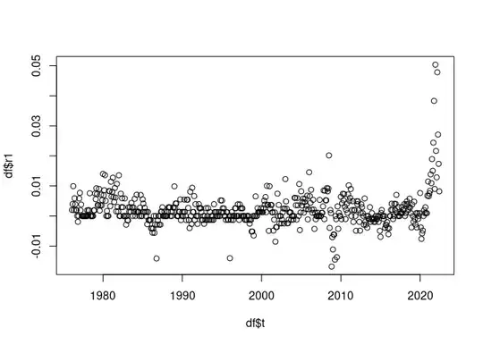
##it makes sense to see the return time series as a time series whose volatility fluctuates around a constant value.
##Given that I am not interested in forecasting the volatility, but the future values of y1, which approach would you suggest?
Forecasting the returns r1 would also be OK, because from them I can easily derive y1.
Would it be possible to use some GARCH model to predict the returns instead of the volatility?
##If possible, I would like a solution relying on the tidymodels paradigm
(https://www.tidymodels.org/) and perhaps its extension for time series
analysis (https://business-science.github.io/modeltime/index.html),
or for GARCH models
(https://albertoalmuinha.github.io/garchmodels/index.html),
but what I need the most is a statistical insight and a bit of code.

^{Created on 2022-08-18 by the reprex package (v2.0.1)}

Answer 1

This is not a time series question. ARIMA or GARCH are completely irrelevant.

There is exactly one question you need to consider, and we can't tell you the answer: what happened at the end of the series, and (a) will the recent increase continue, or (b) does this represent a step change such that the series will go back to a slower increase as before the recent spike from the level now achieved, or (c) is this a one-time effect that will dissipate such that the series will go back to its trajectory before the spike, or (d) something completely different.

Your answer to this question will determine how you model, and it will utterly dominate your forecast. It does not matter at all what autoregressive order you model the rest of the series with if your choice between a-d makes a huge difference in your forecast. Any time series dynamics are of a distant secondary importance to the exactly one question.

Thus: leverage your domain knowledge about what process exactly you are forecasting, what happened recently and what is likely to continue. If you do not have domain knowledge yourself, talk to people who do and get their informed opinion. Yes, that may result in multiple different answers. Consider forecasting multiple scenarios. Ideally, work with whoever consumes your forecast to make decisions and understand the decisions to be made with their tradeoffs.

Related: How to know that your machine learning problem is hopeless?

Answer 2

In addition to Stephan's answer, here are some potentially useful resources for time series forecasting:

• Hyndman & Athanasopoulos - Forecasting: Principles and Practice - A great resource for learning forecasting, all code examples in R
• {fable} - An R package developed by Mitchell O'Hara-Wild, Hyndman, and others, for time series forecasting (used in the above book)
• {modeltime} - An R package for time series forecasting using the tidy principles and the tidymodels framework/workflow

The first resource will help you understand how to think about time series forecasting, how to build good models, and what approaches are appropriate for different issues. The second and third will help you build on that understanding and start building your own models in R, once you're ready.