Distribution change of variables

Question

I'm working on distributions for a physics problem and I am quite stumped on how to proceed properly.

The problem is as follows: I start at the point $(0,0)$ and go a distance $\eta$ in x direction $(\eta, 0)$, from there I go in a random direction $\phi$ (uniformly distributed) a distance $x$ that is gaussian distributed. I need the distribution of $y$, with $y$ being the distance of the resulting point from $(0,0)$

To formalize that:

$f(x)=\frac{1}{b\sqrt{\pi}}\exp(-x^2/b^2)$

(is the distribution of the random x direction) but I also know that

$y = \sqrt{2 x \eta \cos (\phi )+\eta ^2 + x^2}$

with $\phi$ being uniformly randomly distributed between $0, 2\pi$

Is it correct to say (with performing change of variables between x to y, and phi:

$g(y, \phi)\propto f(x)|\frac{dx}{dy}||\frac{dx}{d\phi}|$?

I'm pretty sure this is wrong (I suppose I need the Jacobian in some way), but I can't find good references for it

Answer 1

Let $(X,\Phi,Y)$ be the random variables in question. Let's suppose $X$ and $\Phi$ are independent. $Y$ is a function of those two,

$$Y = f_\eta(X,\Phi)=\sqrt{2X\eta\cos(\Phi) + \eta^2+X^2}$$

for some number $\eta \ge 0.$ (If $\eta \lt 0,$ negating both it and $X$ does not change the distribution of $X$ and places us into the $\eta \gt 0$ situation.) That is, when $X\ge 0,$ $Y$ is the length of the third side of a triangle of side lengths $\eta$ and $X$ with included angle $\Phi;$ and when $X\le 0,$ $Y$ is the length of the third side of a triangle of side lengths $\eta$ and $-X.$ This shows the formula makes sense (we're not trying to find the root of a negative number) and that it is almost everywhere a two-to-one mapping, because

$$f_{\eta}(X,\Phi) = f_{\eta}(-X,\Phi+\pi).$$

The question appears to ask for the joint density function of $(Y,\Phi) = (f_\eta(X,\Phi), \Phi).$

We may easily write the joint density of $(X,\Phi),$ because independence implies the joint density is the product of the univariate densities. The joint probability element therefore is (up to sign)

$$f_{X,\Phi}(x,\phi) = \frac{1}{b\sqrt{\pi}} e^{-x^2/b^2}\,\mathrm{d}x \frac{1}{2\pi}\,\mathrm{d}\phi.\tag{*}$$

To change the coordinates, notice the definition of $Y$ implies

$$y^2 - x^2 - \eta^2 - 2x\eta\cos(\phi)=0.$$

From this we obtain $x$ and $x^2$ (sort of, up to a choice of two solutions) as

$$x = -B(\phi,\eta) \pm \sqrt{\Delta(\phi,\eta,y)}\tag{1a}$$

and

$$x^2 = B(\phi,\eta)^2 + \Delta(\phi,\eta, y) \mp 2B(\phi,\eta)\sqrt{\Delta(\phi,\eta, y)}\tag{1b}$$

where $B(\phi,\eta) = \eta\cos(\phi)$ and $\Delta(\phi,\eta, y) = \eta^2\cos^2(\phi) + (y^2-\eta^2).$

Differentiating (with respect to the variables $(y,x,\phi)$) we also find

$$0 = \mathrm{d}\left(y^2 - x^2 - \eta^2 - 2x\eta\cos(\phi)\right) = 2y\mathrm{d}y - 2x\mathrm{d}x - 2\eta\cos(\phi)\mathrm{d}x + 2x\eta\sin(\phi)\mathrm{d}\phi.$$

Consequently

$$0 = 0\wedge \mathrm{d}\phi = 2y\mathrm{d}y\wedge\mathrm{d}\phi - (2x + 2\eta\cos(\phi))\mathrm{d}x\wedge\mathrm{d}\phi,$$

which we can solve (almost everywhere) to convert the original differential element $\mathrm{d}x\mathrm{d}\phi$ to the new variables,

$$\mathrm{d}x\mathrm{d}\phi = \frac{y}{x + \eta\cos(\phi)}\,\mathrm{d}y\mathrm{d}\phi.\tag{2}$$

Plugging $(2)$ into $(*)$ gives an expression for the joint probability element $f_{Y,\Phi})(y,\phi)\mathrm{d}y\mathrm{d}\phi$ in which "$x$" and "$x^2$" can be replaced by expressions $(1a)$ and $(1b),$ respectively.

Finally, because the map from $(X,\Phi)$ to $(Y,\Phi)$ is two-to-one, we must double the preceding result: that's the answer.

---

I'm not going to work this out further for several reasons. One is that the many-to-one transformation suggests the problem hasn't been stated quite as clearly as it ought to be. Another is that in the question, the expression given for the density of $X$ is incorrect. I have silently fixed it above, assuming the intention is that $X$ have a Normal distribution: but perhaps that's the wrong assumption. A change in the density of $X$ would not change how the answer is worked out, but it would change the details of the final answer. Finally, I suspect that this is just one step in the solution of a problem that, if it were disclosed, might be (much) simpler to solve some other way. Analyzing the density of $(Y,\Phi)$ is not an appetizing prospect.

Answer 2

$$ \begin{aligned} g_Y(y) &=\int_0^{2\pi} \frac{d\phi}{2\pi} \int_{-\infty}^{\infty} dx \frac{1}{b\sqrt{\pi}} \exp(\frac{-x^2}{b^2}) \times \\ & ~~~~~~~~~~~~~~~~~~~~~\times \delta \bigg( y-\sqrt{2x\eta\cos{\phi}+\eta^2+x^2} ~~\bigg) \\ &=\int_0^{2\pi} \frac{d\phi}{2\pi} \frac{1}{b\sqrt{\pi}}\exp{\frac{-\tilde{x}^2}{b^2}}\frac{1} {| \frac{\partial}{\partial x }\sqrt{2x\eta\cos{\phi}+\eta^2+x^2}|_{x=\tilde{x}}|}\\ &\text{where }\tilde{x} \text{ solves } \\ y^2 &= 2\tilde{x}\eta \cos{\phi}+\tilde{x}^2+\eta^2 ~ \\ \end{aligned} $$ Complete the square and solve for $\tilde{x}: y^2=2\tilde{x}\eta\cos{\phi}+\eta^2+\tilde{x}^2$ for $\tilde{x}$ in terms of $\phi, y,$ and $\eta$. And now the work begins . . .

But the integral looks vaguely familiar. $\sqrt{2x\eta\cos{\phi}+\eta^2+x^2} $ is screaming out to be $Y=|X+\eta|_2$, or the distribution of the Euclidean length of $X+\eta$ where $X$ and $\eta$ are in $\mathbb{R}^d$ and $\phi$ is simply the angle between them. It suggests that there is an earlier statement of this problem that might yield geometrical transformation and a much easier problem to solve. Maybe not, but you never know.

Answer 3

Whuber gave an answer to the question about the coordinate transformation. But in the final two sentences of his answer he noted

Finally, I suspect that this is just one step in the solution of a problem that, if it were disclosed, might be (much) simpler to solve some other way. Analyzing the density of $(Y,\Phi)$ is not an appetizing prospect.

In your recent edit you disclosed that you are not after the joint distribution $f_{Y,\Phi}(y,\phi)$ but instead after the marginal distribution $f_Y(y)$.

In this answer we show one of those other more simple ways how to solve it without directly tackling the solution for the joint density distribution.

---

When I reverse engineer this, then I can model this as the distance $y$ between the origin and a random point on a circle with radius $\eta$ and midpoint $(0,x)$ where $x$ follows a normal distribution with standard deviation $b$.

Instead of computing the distribution density it might be easier to compute the cumulative distribution.

We can consider the values of $x$ and $\phi$ for which the point on the circle is still below a distance $y$ (ie. $f(x,\phi)<y$) and integrate over that area.

We can do this by considering for every point $x$ how much of the circle of radius $\eta$ centered at $0,x$ is intersecting with the circle of radius $y$ centered at $0,0$. Then integrate over all $x$ while multiplying with the fraction of the circle that intersects inside the circle of radius $y$.

$$F(Y<y) = 2 \int_{max(\eta-y,y-\eta)}^{y+\eta} \frac{1}{b\sqrt{\pi}} e^{-\frac{x^2}{b^2}} \overbrace{\frac{1}{\pi} cos^{-1}\left(\frac{x^2+\eta^2-y^2}{2x\eta}\right)}^{\text{fraction of circular segment intersecting}}dx + 2\int_0^{max(0,y-\eta)} \frac{1}{b\sqrt{\pi}} e^{-\frac{x^2}{b^2}} dx$$

To get the distribution density you differentiate the above. For this you can use Leibniz integral rule and you will get several terms because not only the integrand is dependent on $y$ but also the integration limits (but since the integrand is zero at the limits, or cancels, these terms will be zero as well).

If I do this then I get to

$$f(y) = 2 \int_{abs(y-\eta)}^{y+\eta} \frac{1}{b\sqrt{\pi}} e^{-\frac{x^2}{b^2}} \frac{1}{\pi} \frac{y}{x\eta}\frac{1}{\sqrt{1-\left(\frac{x^2+\eta^2-y^2}{2x\eta}\right)^2}}dx $$

or

$$f(y) = \frac{y}{b\pi^{3/2}} \int_{abs(y-\eta)}^{y+\eta} e^{-\frac{x^2}{b^2}} \frac{1}{\sqrt{x^2-(y-\eta)^2}\sqrt{(y+\eta)^2-x^2}}dx $$

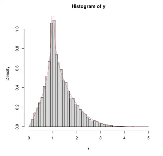
Demonstration with computational simulation

Below is a histogram for a simulation of size $n=10^4$ with parameters $\eta= 1$ and $\sigma = b/\sqrt{2} = 1$. Superimposed is a computation of the density distribution based on a differentiation of the formula above.

### settings
set.seed(1)
n = 10^4
eta = 1
sig = 1
simulate and plot histogram
phi = runif(n,0,2pi)
x = rnorm(n,0,sig)
y = sqrt(eta^2+x^2+2xetacos(phi))
hist(y, freq=0, breaks = seq(0,5,0.1))
integrand function
integrand = function(x,z) {
    ### exit for special cases to prevent NA values for acos
    if (x-eta>=z) {
      return(0)
    }
    if (x+eta<=z) {
      return(dnorm(x,0,sig))
    }
    return(dnorm(x,0,sig)acos((x^2+eta^2-z^2)/(2x*eta))/pi)
}
integrand = Vectorize(integrand)
compute density by integrating integrand
pcomp = function(z) {
 d = 0.001
 xi = seq(abs(z-eta),z+eta,d)
 2sum(integrand(xi,z))d + 2*(pnorm(max(0,z-eta))-0.5)
}
pcomp = Vectorize(pcomp)
compute cumulative distribution and differentiate for density
dd = 0.05
zs = seq(0,5,dd)
lines(zs[-1]-dd/2,diff(pcomp(zs))/dd,col=2)