The integral can be understood in the Riemann-Stieltjes sense.
Background
This is a natural generalization of the usual (elementary) Riemann integral with respect to the variable $x.$ Recall that such an integral, when it exists, can be approximated as accurately as you might wish by Riemann sums: you partition the interval of integration (call it $[a,b]$) into sufficiently short pieces, which will be the bases of rectangles, and use the values of the integrand within those intervals for the (signed) heights of rectangles and add up all the rectangle areas.
More specifically, letting the points in the interval be
$$a = t_0 \lt t_1 \lt \cdots \lt t_N = b,$$
where every $t_{i+1} - t_i$ is smaller than some tiny value $\delta,$ you can select any points $t_i{*} \in [t_i, t_{i-1}]$ for computing the rectangle heights $\psi(t_i^*).$
The Riemann-Stieltjes integral, when it exists, is more often written in the form
$$\int_a^b \psi(x)\,\mathrm{d}F(x)$$
where $F$ is increasing and right-continuous (as are all probability functions). This means that instead of using the interval widths $t_{i+1}-t_i$ for the bases of the rectangles, you will weight them by the values of $F,$ using $F(t_{i+1}) - F(t_i)$ for the bases. In effect, $F$ is trying to tell you how much weight to assign to any possible interval $[t_i, t_{i+1}]$ in the integral. When $F$ is a distribution function then, by definition, $F(t_{i+1}) - F(i)$ is the probability of the interval $(t_i, t_{i+1}]$ and the approximation is the familiar sum of values of $\psi$ multiplied by (approximate) probabilities: it's an expectation.
Application
A dataset $(x_1, x_2, \ldots, x_n)$ gives rise to a random variable $X$ in a natural, physical way: take $n$ slips of paper ("tickets"), write $x_i$ on the $i^\text{th}$ ticket, put them all into a box, blindly withdraw a single ticket from that box, and read its value. Because (at least in theory) every ticket has an equal chance of being withdrawn, each ticket has a chance of $1/n.$
By definition, the distribution function of $X$ is
$$F_X(x) = \Pr(X \le x) = \left(\text{number of } x_i \text{ not exceeding } x\right)\times \frac{1}{n}.$$

The black dots and lines plot $F_X$ for the dataset $(1, 2, 2, 2, 4, 4).$ The dataset is depicted by the red points below the horizontal axis.
To evaluate a Riemann-Stieltjes integral we will be considering the weighted differences $F(t_{i+1}) - F(t_i)$ for arbitrarily short intervals $[t_i, t_{i+1}]\subset [a,b].$ These values equal (a) the number of data points less than or equal to $t_{i+1}$ (b) minus the number of data points less than or equal to $t_i$ (c) times their common probability of $1/n.$ Clearly the net of the counts (a) and (b) is *the number of data points in the interval $(t_i, t_{i+1}].$ Consequently,
The only intervals $(t_i, t_{i+1}]$ contributing to the Riemann-Stieltjes integral are those that include at least one of the data $x_j.$

The dotted vertical lines indicate a partition of the interval $[a,b]=[0,5].$
Thus, any approximation to this integral is a sum over tiny intervals surrounding the data points; and the value contributed by such an interval is (a) the count of data points in that interval (b) times $1/n$ (c) times the value of $\psi$ at some arbitrary point in that interval.
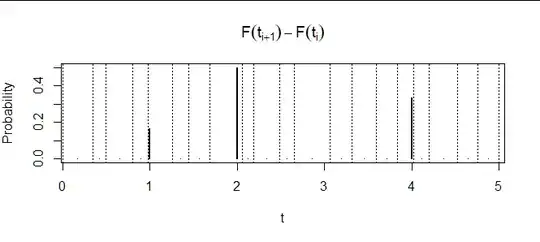
This figure plots the differences of $F$ against values of $t_i^*$. In effect it reproduces the information given by the red points in the first figure: it shows where the data values occur and with what multiplicities.
Suppose, now, that $\psi$ is continuous. This means the values of $\psi$ within tiny intervals do not vary much compared to the sizes of those intervals. This assumption permits us to approximate the Riemann-Stieltjes approximation (!) by choosing the specific values $\psi(x_j)$ for $x_j\in(t_i,t_{i+1}].$
At this point we make an algebraic move to simplify everything. Suppose $(t_i, t_{i+1}]$ is an interval that is so small it contains only one unique data value. However, that value might appear multiple times in the dataset. If it appears $s$ times, it will be the values of the data points $x_{j_1}=x_{j_2}=\ldots=x_{j_s},$ say. Each of these is our chosen representative $t_i^*.$ The contribution of this interval to the integral therefore is
$$\psi(t_i^{*}) \left(F(t_{i+1}) - F(i)\right) = \psi(x_{j_1}) \times \left(s\times \frac{1}{n}\right) = \sum_{k=1}^s \psi(x_{j_k})\times \frac{1}{n}.$$
That is, each data point $x_j$ contributes a value of $\psi(x_j)$ times a probability of $1/n$ to the integral.
The resulting approximation to the integral is
$$\int_{a}^b \psi(x) \,\mathrm{d}F(x) \approx \sum_{j=1}^n \psi(x_j) \frac{1}{n} = \frac{1}{n}\sum_{j=1}^n \psi(x_j).$$
In the limit of arbitrarily small intervals, this sum equals the integral (by definition).
Finally, the indefinite integral in the question is implicitly meant to extend over all real numbers. This is defined to be the limit of the integrals over finite intervals $[a,b]$ as $a$ and $b$ (separately) tend to $-\infty$ and $\infty.$ It should be clear from the foregoing result that once $a$ is smaller than the minimum data value and $b$ is larger than the maximum data value, the integral no longer changes and its limiting value has been reached.


