The contrast (i.e., estimand) of interest in diff-in-diff is $\color{red}{E[Y^1_{post}|A=1]} - \color{blue}{E[Y^0_{post}|A=1]}$, which relies on the unobserved quantity $\color{blue}{E[Y^0_{post}|A=1]}$. How can we get this quantity if it is unobserved?
The parallel trends assumption is a counterfactual assumption about $\color{blue}{E[Y^0_{post}|A=1]}$, the mean potential outcome in the post-period for the treated units had they instead received control. The assumption can be stated as follows:
$$\color{blue}{E[Y^0_{post}|A=1]}-\color{green}{E[Y^0_{pre}|A=1]} = \color{darkorange}{E[Y^0_{post}|A=0]}-\color{brown}{E[Y^0_{pre}|A=0]}$$
The quantity on the left is the trend in the potential outcomes under control (i.e., difference between outcomes post and pre) for the treated units, and the right side is the trend in the potential outcomes under control for the control units. The parallel trend assumption states that these two trends are equal (i.e., parallel if plotted). See the graph below, which colors the dots corresponding to the quantities they represent:
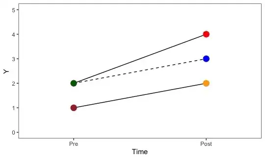
The dotted line represents the counterfactual trend under control for the treated units. The solid lines represent the observed trends. The parallel trends assumption is that the dotted line is parallel with the bottom solid line.
The assumption is fundamentally untestable because there is no data for $\color{blue}{E[Y^0_{post}|A=1]}$; for the treated units in the post-period, we only observe their potential outcomes under treatment (i.e., $\color{red}{E[Y^1_{post}|A=1]} = \color{red}{E[Y_{post}|A=1]}$).
It is important to note that the terms on the right side are observed; they are simply the observed outcome means in the control group before and after treatment. We still don't have $\color{green}{E[Y^0_{pre}|A=1]}$; to get this, we need the assumption
$$
\color{green}{E[Y^0_{pre}|A=1]} = \color{green}{E[Y^1_{pre}|A=1]}
$$
That is, the pre-period outcomes don't depend on the treatment you end up receiving (i.e., because the future can't affect the past). This quantity is also observed; it's just the average outcome in the treated group in the pre-period.
So now, thanks to the parallel trends assumption, we can write
\begin{align}
\color{blue}{E[Y^0_{post}|A=1]} &= \color{green}{E[Y^0_{pre}|A=1]} + \color{darkorange}{E[Y^0_{post}|A=0]} - \color{brown}{E[Y^0_{pre}|A=0]} \\
&= \color{green}{E[Y^1_{pre}|A=1]} + \color{darkorange}{E[Y^0_{post}|A=0]} - \color{brown}{E[Y^0_{pre}|A=0]} \\
&= \color{green}{E[Y_{pre}|A=1]}+\color{darkorange}{E[Y_{post}|A=0]}-\color{brown}{E[Y_{pre}|A=0]}
\end{align}
where the last line is made up solely of observed quantities.
Finally, we can write the counterfactual estimand as
\begin{align*}
\color{red}{E[Y^1_{post}|A=1]} - \color{blue}{E[Y^0_{post}|A=1]} &= \color{red}{E[Y_{post}|A=1]} - \\
& \qquad (\color{green}{E[Y_{pre}|A=1]} + \color{darkorange}{E[Y_{post}|A=0]} - \color{brown}{E[Y_{pre}|A=0]}) \\
&= (\color{red}{E[Y_{post}|A=1]} - \color{green}{E[Y_{pre}|A=1]})- \\
& \qquad (\color{darkorange}{E[Y_{post}|A=0]}-\color{brown}{E[Y_{pre}|A=0]})
\end{align*}
which is precisely the diff-in-diff observed variables estimand. That is, to be able to write the counterfactual estimand as a contrast among observed quantities, we need the parallel trends assumption because it links the counterfactual quantities to the observed quantities. It is an essential assumption for diff-in-diff and the whole motivation behind the methodology. In theory it's a much more plausible assumption than strong ignorability or the exclusion restriction for instrumental variables, which is why diff-in-diff is such a powerful method.
