The Importance of the Your Prior's Variance or "Range"
The answer you used as a guide makes two points about the distribution it selected as a prior, one about the distribution's mean and a second about the distribution's variance, spread, or "range":
"I came up with these parameters for two reasons:
The mean is $\frac{\alpha}{\alpha + \beta} = \frac{81}{81+219} = .270$
As you can see in the plot, this distribution lies almost entirely within (.2, .35)- the reasonable range for a batting average."
The author selected that range because it closely approximated the actual historical variation among professional baseball players. He plots the distribution, but I will replot it here to show exactly where the average, bottom 1%, and top 1% of players fall on his prior distribution:

So 98% of players fall between .213 and .332 on his prior distribution.
Contrast that range with the expected range implied by your Group 1 prior:

Your prior for Group 1 suggests that the difference between the top 1% and bottom %1 is less than half of the range his prior expects.
Why is yours so different? Two reasons: 1) the total count for your Group 1 prior is 500, whereas the total count for his prior is only 300 and 2) your prior reflects much lower mean percentages than his, which further reduces the variance (if you consult the formula for the variance of a Beta distribution, you will see that for a given count, mean values closer to .5 result in significantly larger variances than more extreme mean values). The net effect is that your priors impose much stronger assumptions than his about the range of abilities you expect. Your prior for Group 2 reflects a similarly small range of expected variation:

Some Simple Ways to Increase Your Expected Range of Abilities
One way to widen your expected range of abilities to be more like his would be to cap your count at 300, as he does, while maintaining the same mean. For Group 2, your prior would then look like this:

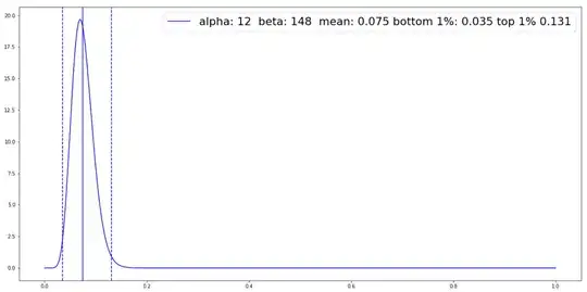
If you wanted, you could further reduce your count to 160, which would result in a range of abilities almost as wide as his:
The Posterior Mean as a Weighted Combination of the Data's Mean and the Prior's Mean
To fully understand why your estimate for Player B-1 was so high, though, you need to understand how the count of the prior and the count of observed data both influence the mean of the posterior distribution (your estimate). Fortunately, there is a simple formula that enables us to understand the mean of the posterior distribution as a weighted combination of the mean of the data and the mean of the prior. In your example, that formula works as follows:
total count of data = 1 hit + 55 misses = 56
mean of data = .0117
total count of prior = 30 hits + 471 misses = 501
mean of prior = .0599
total count of posterior = (30 + 1) + (471 + 55) = 557 total
fraction of posterior from data = 56 / 557 ~ .10
fraction of posterior from prior = 501 / 557 ~ .90
mean of posterior = (fraction from data) * (mean of data) + (fraction from prior) * (mean of prior)
.055 ~ .10 * .0117 + .90 * .0599 [truncating for readability]
Your posterior estimate for Player B-1 (.055) was high relative to his actual observed data (.0117) because your Group 1 prior's count (501) and your prior's proportional influence on the posterior distribution (.9) was roughly nine times greater than the data's count (56) and the data's proportional influence on the posterior (.1). Lowering your prior's count to 160 would alter your result as follows:
total count of prior = 12 hits + 148 misses = 160
mean of prior = .0599 [unchanged]
total count of posterior = (12 + 1) + (148 + 55) = 216 total
fraction of posterior from data = 56 / 216 ~ .26
fraction of posterior from prior = 160 / 216 ~ .74
.047 ~ .26 * .0117 + .74 * .0599 [truncating for readability]
Although the posterior's mean remains more strongly influenced by the prior than by the data, the prior is now only three times as influential instead of nine times. As a result, your posterior estimate is "pulled" less powerfully toward the prior's mean: .0599. The prior is exerting less influence than before because its lowered count makes it less surprised by poor hitters. (To shift the expected "lowest 1%" downward and the expected "highest 1%" upward, we lowered the count of our prior from 500 to 160.)
A More Sophisticated, Empirical Solution to Establish the Variance of Each Group's Prior
Instead of arbitrarily adjusting the strength or count of your prior to get a range that seems reasonable, a more rigorous methodology would be to learn the variance of the prior distribution for each group directly from your data. To do this, you would fit the prior for Group 1 to the actual percentages for all the players in that group using either moment matching or maximum likelihood estimation (MLE). Moment matching could be performed by hand a data set this small and would likely not differ much from what you would get fitting them through MLE. You have already calculated the mean (first moment) for each group, so you would just need to calculate the variance (second moment) for each group and then solve for each prior's $\alpha$ and $\beta$ parameters based on the expected mean and expected variance for each group of hitters. The point is: we can estimate the variance within each group/population based on the variance we have observed within our samples from each group, and use that information to sculpt more sensible priors.


