First of all, I guess we can agree that if different statistical methods give the same results for the same data, it's a kind of good, isn't it? It means that there's nothing fancy about the data or the methods.
Second, you are not using any prior. Technically, you could consider this code to be implicitly using an "uninformative" Haldane prior, i.e. one with $\alpha=\beta=0$ in a beta-binomial model. Such prior would soon get overwhelmed with the data and give results nearly the same as when maximizing the likelihood function alone.
The posteriors would have the expected values $E[A] = H(A)/N$ and $E[B] = H(B)/N$ respectively. In your two-sample $z$-test you are comparing the difference between $H(A)/N$ and $H(B)/N$ as well, so looking at the same thing. Recall that $E[A] - E[B] = E[A - B]$, so otherwise that you are using a normal approximation in the second case, you expect them to be the same.
The results are so close because of three things that hold: (a) the prior is very "weak", so it has a small influence on the result, (b) the sample size N is relatively big, so it overwhelmed the prior, and (c) because of sample size is relatively big, the normal approximation works quite well. If you tried something like N=5 the differences would be more clear. Notice however that while both approaches gave similar results, they are based on completely different assumptions and have different interpretations, so in general, should not be thought of as exchangeable.
Code example
Below you can see your code modified so that it also produces the plots of the beta distributions vs the normal approximations.
from scipy.stats import beta, norm
import numpy as np
import matplotlib.pyplot as plt
np.random.seed(42)
N = 5
R = 10
sample_size = 100_000
def beta_std(α, β):
    v = (α * β) / ((α + β)*2  (α + β + 1))
    return np.sqrt(v)
for H_A, H_B in zip(np.random.randint(1,N,R), np.random.randint(1,N,R)):
a_beta = beta(H_A, N-H_A)
b_beta = beta(H_B, N-H_B)
prob = (a_beta.rvs(sample_size) > b_beta.rvs(sample_size)).mean()
z = (H_A/N - H_B/N)/np.sqrt((H_A/N*(1-H_A/N)/N) + (H_B/N*(1-H_B/N)/N))
print(round(prob, 3), "\t", round(norm.cdf(z),3))

x = np.linspace(0, 1, 500)
fig, (ax1, ax2) = plt.subplots(1, 2)

mean_A = H_A/N
std_A = beta_std(H_A, N-H_A)

ax1.plot(x, a_beta.pdf(x), label="beta")
ax1.plot(x, norm(loc=mean_A, scale=std_A).pdf(x), label="normal approx")
ax1.set_title(f"H(A)={H_A}")
ax1.legend()

mean_B = H_B/N
std_B = beta_std(H_B, N-H_B)

ax2.plot(x, b_beta.pdf(x), label="beta")
ax2.plot(x, norm(loc=mean_B, scale=std_B).pdf(x), label="normal approx")
ax2.set_title(f"H(B)={H_B}")
ax2.legend()
With a small sample size N=5, the approximation is not perfect:

However, if you increase it to N=100, it is very close:
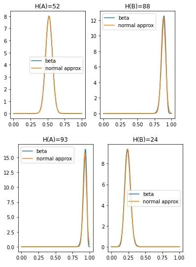
No wonder you get nearly the same results. More than this, the distribution of the difference between the random variables is even better approximated by a normal distribution, not to unnecessarily extend the answer, I made a notebook illustrating this.

