Joint negative log-likelihood of the Binomial model $\mathrm{Binomial}(n, p)$ with unknown $n$ and $p$

Question

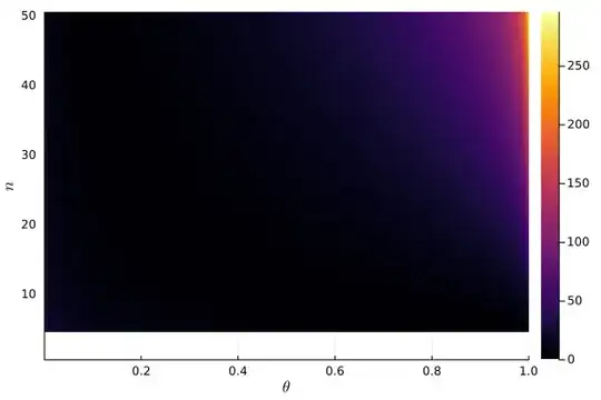
I'm trying to make sense of the following plot portraying the joint negative log-likelihood for the Binomial model $\mathrm{Binomial}(n,p)$ with unknown $n$ and $p$ and $y=5$. Note that the white part indicates a negative log-likelihood equal to minus infinity due to the fact that $n$ must be at least $y=5$. Also, I put an arbitrary cutoff at $n=50$.

The joint likelihood (still evaluated at $y=5$) has a clear maximizer while the negative log-likelihood has not.

Is it correct to say that this is the case because the joint likelihood is not log-concave?

---

Julia code to reproduce the plots above.

using Plots, StatsPlots, Distributions, LaTeXStrings, Random
Random.seed!(1994)
joint likelihood of n ad θ
begin
    ns = 1:50
    θs = range(0., stop=1., length=1000)
    A = zeros(length(ns), length(θs))
    for (i, n) in enumerate(ns), (j, θ) in enumerate(θs)
        A[i, j] = pdf(Binomial(n, θ), 5)
    end
    heatmap(A, xlabel=L"\theta", ylabel=L"n", xformatter=x->"$(x/length(θs))")
    savefig("plots/joint_likelihood.png")
end
joint negative log-likelihood of n ad θ
begin
    ns = 1:50
    θs = range(0., stop=1., length=1000)
    A = zeros(length(ns), length(θs))
    for (i, n) in enumerate(ns), (j, θ) in enumerate(θs)
        A[i, j] = -loglikelihood(Binomial(n, θ), 5)
    end
    heatmap(A, xlabel=L"\theta", ylabel=L"n", xformatter=x->"$(x/length(θs))")
    savefig("plots/joint_neg_loglikelihood.png")
end

Answer 1

We can use profiling to make our lives easier here: the idea is that maybe we can't easily solve for $\max_{n,\theta} L(n, \theta \mid y)$ but for each particular $n$ we can find the $\theta$ that maximizes $L$, and then we can optimize that over $n$.

So let $L(n, \theta \mid y) = {n\choose y} \theta^y(1-\theta)^{n-y}$ be the likleihood that we're looking to maximize. The log likelihood is therefore $$ \ell(n,\theta\mid y) = y\log\theta + (n-y)\log(1-\theta) + \log{n\choose y}. $$ For each $n$ we can optimize this over $\theta$ by taking derivatives, which gives the usual MLE of $\hat\theta_n = \frac y n$.

This means that the profiled log likelihood is $$ \ell_p(n\mid y) = \ell(n, \hat\theta_n\mid y) = y\log (y/n) + (n-y)\log(1-y/n) + \log {n\choose y} $$ and we want to understand the maximum of this. To recap, if we think of the set of all valid $(n,\theta)$ pairs, this says that within each slice corresponding to a particular $n$ we know the maximum value of $\ell$ or $L$ will occur at $(n, \hat\theta_n)$. If we then optimize over each of these slice extrema, which now just depend on $n$, we will get the global optimum.

Using $0\cdot \log 0 = 0$ we can see that $$ \ell_p(y\mid y) = y \log 0 + 0\cdot \log 0 + \log 1 = 0 $$ and since the original likelihood is discrete, we know that it's bounded above by $1$ ,which means a log likelihood of zero is as big as we can get. This shows that if we are allowed to vary both $n$ and $\theta$ we will choose to set $n=y$ and $\hat\theta=1$ which makes the particular value we observed as likely as possible, i.e. it would happen with probability $1$.

That's often the trouble with doing this kind of joint optimization. We're basically able to vary both the mean and the variance and so we can make the particular sample that we got as likely as possible.

I'm not very familiar with Julia so I'm not sure if your plots are correct but this at least is the behavior that you should be seeing. It looks like the second plot shows this. Also we know that $(n, y/n)$ is the optimal point for each value of $n$ so that explains the $1/x$-looking shape in the second plot as well, starting at the maximum of $(y, 1)$ and fading away along the curve $(n, y/n)$.