4

In the following paper, https://users.nber.org/~rdehejia/papers/matching.pdf, it says:

Matching with replacement involves a tradeoff between bias and variance. With replacement, the average quality of matching increases; thus, the bias decreases but the variance increases.

Why is it that the variance increases? Is there a simple and intuitive way to understand this? I understand the reuse of control units results in less information being used, but is there a mathematical or intuitive way to understand the link from this to the higher variance? Thanks.

Richard Hardy
  • 67,272
user321627
  • 4,474

2 Answers2

4

I can offer two answers, one intuitive but somewhat unsatisfying and the other statistically rigorous but (to me) somewhat opaque.

The first comes from a measure known as the effective sample size (ESS) of a weighted sample, which is the approximate size of an unweighted sample that carries the same information as the weighted sample in question. One can estimate the ATT after matching with replacement by assigning weights to each control unit equal to the total number of times that control unit is matched (it's a little more complicated when matching more than one control unit per treated unit). Given these weights, we can compute the ESS of the control sample as $$ ESS = \frac{(\sum w)^2}{\sum w^2} = \frac{n}{1 + \text{Var}(w^*)}$$ where $w_i^* = \frac{w_i}{\bar{w}}$. The greater the variability of the weights, the lower the ESS is, so the lower the precision of the estimate of the control potential outcomes mean is.

The more technical answer comes from Abadie & Imbens (2006, p246-247), who derive the asymptotic variance of matching estimators. A term in the numerator of the variance of the ATT (and there is a similar term in the variance of the ATE) is $$\sum\limits_{i=1}^N \left(W_i-(1-W_i)\frac{K_M(i)}{M} \right)^2 \sigma^2(X_i,W_i)$$ where $W_i=1$ if the unit is treated and $0$ otherwise and $K_M(i)$ is the number of times unit $i$ is used as a match, $M$ is the number of matches per treated unit, and $\sigma^2(X_i, W_i)$ is the variance of the potential outcome residual, which we'll assume is constant here so we can ignore it. Because of the square, if any control unit were to be matched more than once, this component of the variance would be higher than if all control units were matched at most once.

Consider a simple example with two control units and two treated units and 1:1 matching (so $M=1$). If both control units were matched once (i.e., each to one treated unit), the variance component contribution of the control units ($W_i=0$) would be $(-1)^2 +(-1)^2 = 2$. If one were matched zero times and the other were matched twice, the component would be $(0)^2 + (-2)^2 =4$. So, clearly, by reusing control units when matching with replacement, the variance increases relative to matching each unit only once.


Abadie, A., & Imbens, G. W. (2006). Large Sample Properties of Matching Estimators for Average Treatment Effects. Econometrica, 74(1), 235–267. https://doi.org/10.1111/j.1468-0262.2006.00655.x

Noah
  • 33,180
  • 3
  • 47
  • 105
2

I'm not sure I understand details of your 'matching' procedure. However, a binomial distribution (with replacement) has larger variability than a corresponding hypergeometric distribution (without replacement). Intuitively, as sampling without replacement depletes the population, the variability of available choices decreases.

Example: Consider the number of red chips in five draws, sampling with replacement (binomial) from an urn with 5 red chips and 5 green chips. By contrast, consider sampling without replacement (hypergeometric). The two distributions are plotted below. The binomial standard deviation is $1.1180$ and the hypergeometric SD is $0.8333.$

x1 = 0:5;  n = 5;  p = 0.5
b.pdf = dbinom(x1, n, p)
x2 = 0:5;  n = 5;  r = 5; b = 5
h.pdf = dhyper(x2, r,b, n)

enter image description here

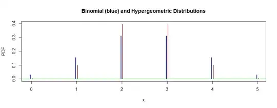
hdr = "Binomial (blue) and Hypergeometric Distributions"
plot((0:5)-.02, b.pdf, ylim=c(0,.4), ylab="PDF", xlab="x", 
     type="h", lwd=2, col="blue", main=hdr)
 lines((0:5)+.02, h.pdf, type="h", lwd=2, col="brown")
 abline(h=0, col="green2")

Below each of the experiments is simulated 10,000 times and results are summarized.

set.seed(2021)
x1 = rbinom(10^4, 5, .5)
summary(x1); sd(x1)
   Min. 1st Qu.  Median    Mean 3rd Qu.    Max. 
  0.000   2.000   3.000   2.515   3.000   5.000 
[1] 1.123965   # aprx binomial SD
x2 = rhyper(10^4, 5,5, 5)
summary(x2); sd(x2)
   Min. 1st Qu.  Median    Mean 3rd Qu.    Max. 
  0.000   2.000   3.000   2.497   3.000   5.000 
[1] 0.8397981
BruceET
  • 56,185