Strange results from t-student cdf with "Abramowitz" approximation

Question

I need to evaluate a large number of Cumulative Distribution Functions of Student's t distributions. I'm calculating the Student's t distribution using the approximation stated in "Abramowitz and Stegun. Handbook of Mathematical Functions." book, at this page: http://people.math.sfu.ca/~cbm/aands/page_949.htm

$$ A(t|v) \approx 2 P(x) -1, \; \; \; x = \frac{t(1-\frac{1}{4v})}{\sqrt{1+\frac{t^2}{2v}}} $$

Where:

• $A(t|v) $ is the cdf of the Student's t
• $t$ is the Student's t random variable for the Student's t distribution
• $v$ are the degrees of freedom of the Student's t
• $P(x)$ is cdf of the Gaussian distribution
• $x$ is the random variable for the Gaussian distribution

I'm approximating the gaussian cdf too; the approximation formula is took from Abramowitz book too at this page: http://people.math.sfu.ca/~cbm/aands/page_932.htm (formula $26.2.19$)

The problem is that the values of the Student's t cdf I'm receiving are all negative. The reason for this is that all the values of the Gaussian cdf ($P(x)$) I'm obtaining are very low (for example: $0.1029537234175692291112889$), so the quantity $A(t|v) \approx 2P(x)-1$ is always negative... I don't know if it's important, but the amount of my degrees of freedom is about $1023$ or very similar to it.

Someone knows why this approximation from the Abramowitz doesn't seem to work?

Answer 1

$A(t|v)$ is not the CDF, it's the probability of a Student's t variable being smaller than $t$ in absolute value (i.e. the "area" between $-t$ and $t$, that's why it's called $A$). Because of this, the approximation is understood to hold for $t > 0$, hence where $x$ is positive as well, and so $P(x) > 0.5$, and $A(t|v) > 0$. You are simply using the approximation where it is not valid (or meaningful).

If you have $v = 1023$ (which is very high), the normal approximation (just use the normal CDF) may be sufficient for your purposes.

Edit to clarify alternatives:

What I'm suggesting is either that you use:

1. The normal approximation, where you would just compute $P(t)$, where $P$ is an approximation to the normal CDF.
2. Approximation 26.7.10 from Abramowitz & Stegun, which is a small correction where you first compute $x = \frac{t(1-\frac{1}{4v})}{\sqrt{1+\frac{t^2}{2v}}}$, and then compute $P(x)$, instead of $P(t)$.

For large $v$, $x \approx t$, that's true, but this small correction does make a difference.

Below, some R code that describes both methods and compares to R's built-in pt function, which approximates the Student t CDF:

v <- 1023
t <- seq(-10,0,length.out = 100)

# R's approximation to the CDF
cdf.R <- pt(t,v)

# The normal approximation, P(t)
cdf.normal_approx <- pnorm(t)

# The Abramowitz & Stegun correction, P(x)
x <- t * (1-1/(4*v))/sqrt(1+t*t/(2*v))
cdf.as_approx <- pnorm(x)

# Plot the error
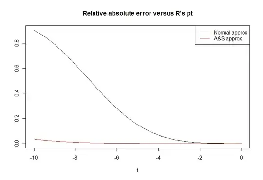
plot(t, abs(cdf.R-cdf.normal_approx)/cdf.R,main="Relative absolute error versus R's pt",type="l",ylab="")
lines(t,abs(cdf.R-cdf.as_approx)/cdf.R,col="red")
legend("topright",legend = c("Normal approx","A&S approx"),col = 1:2,lwd=1)

You can see in the plot below that the second option appears to produce smaller error. I'm not sure which algorithm R uses, but if you don't have a built-in equivalent in whatever tool you are using, the A & S approximation 26.7.10 will do the trick (especially since you have already coded most of it...)