This is not a proper solution, but since no one else has answered in 8 years, I thought it would be useful to offer some intuition, as well as a pragmatic approach, just in case some one else needs it or can build off of it.
Motivation
I came across this problem since I was using fractal brownian motion (FBM) for procedural terrain generation. Inigo Quilez gives a description of FBM here. I needed FBM for its spatial patterns but also needed results to match the hypsography of the Earth. If I knew the CDF of FBM, then I could map the results of FBM to a quantile, and then pass that quantile to the inverse CDF for the hypsography of the Earth. This would achieve the desired spatial patterns while also matching the hypsography of the Earth. Since FBM is a linear combination of several uniform variables, the answer to this stack overflow question is the PDF of FBM.
Building Intuition
Let's first discuss the Irwin-Hall distribution and then see if it can generalize to linear combinations. Philip (1927) gives an explanation of the Irwin-Hall distribution and he includes some intuition in his explanation. Another good article I found is Marengo et al.(2017), who provides some geometric intuition. I think the key insight is that, for a given value of $z$, the Irwin-Hall distribution counts the number of "ways" that $z$ can occur as the sum of $n$ independent and uniformly distributed variables.
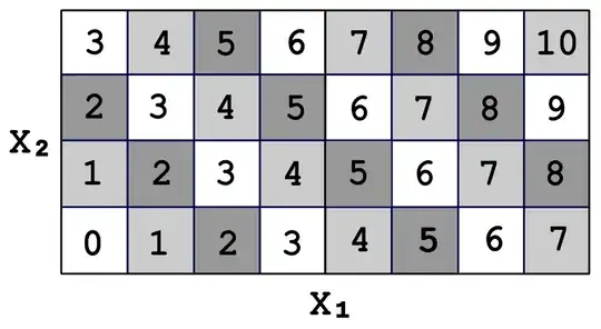
Let's consider a simple discrete case that approximates the Irwin-Hall distribution. Let's say there are 2 variables that are independent and uniformly distributed. Each variable can take on the value of any whole number from 0 to 3, inclusive. We can write out a table that describes all the possible ways this situation could play out:

The value "2" occurs 3 times out of 16. This can be seen forming a diagonal line of cells. Since each occurrence is equiprobable, the probability that $Z=2$ is 3/16.
If we increase the number of values that our variables can assume, and then scale these values to the range $[0,1]$, then we are left with a better approximation for the Irwin-Hall distribution. As the number of possible values increases to infinity, the Irwin-Hall distribution results. If we want to consider the Irwin-Hall distribution for more random variables, then we simply add more dimensions to our table. Since there are infinitely many cells in our table, the table can be treated as an n-dimensional hypercube. Each side of the hypercube is a axis-aligned halfspace. The region where the value "$Z<z$" results can be treated as a diagonally-aligned halfspace. The region where the value "$Z=z$" results can be treated as a flat $n-1$ dimensional subspace (e.g. a line for $n=2$, a plane for $n=3$, etc.). The probability density for the Irwin-Hall distribution is the magnitude of the intersection between the axis-aligned halfspaces and the diagonal subspace (e.g. length for $n=2$, area for $n=3$). The cumulative density is the magnitude for the intersection of all halfspaces. We'll denote this magnitude $V$.

Generalizing for Linear Combinations: Practical Examples
We can use this intuition to extend the Irwin-Hall distribution to account for any linear combination of uniform variables. If one of the dimensions of our table is cropped, but we scale by the same factor as before, then the range for that dimension will not be $[0,1]$ but something else, denoted $[0,c_k]$. This is effectively the same as if OP's linear combination were set so that $c_k=1$ for all but one $k$. The PDF for this linear combination is still the magnitude of a flat $n-1$ dimensional subspace, however instead of that subspace intersecting a n-dimensional hypercube, it intersects a n-cell (the n-dimensional generalization of a rectangle). We can generalize this to say that any linear combination of uniform variables can be described by an n-cell whose dimensions are $c_1,c_2,\ldots,c_n$
[NOTE: we will assume for now that $c_k \geq 0$ for each $k$]
We notice a pattern. There are certain regions of the table. Within a region, the gradient of the probability density is a constant. To illustrate, if $X_1=3$ and $X_2=1$, then the number of cells where $Z=X_1+X_2$ will not change as we increment $X_1$ or $X_2$. We will color code these regions:

This explains something we notice when we simulate such a distribution in R:
N=1e7; hist(runif(N)+runif(N)/2)

In this case, $c_1=1$ and $c_2=\frac{1}{2}$. Situations where $Z\in[\frac{1}{2},1]$ are equiprobable. This occurs because if $Z$ were one of these values, then it would have to occur because we occupy a region where any change to a $X$ variable will not affect the magnitude of the intersection between the n-cell and the subspace where $Z=z$.
The effect becomes more subtle when we increase $n$, but never truly goes away:
N=1e7; hist(runif(N)+runif(N)/2+runif(N)/4)

When we illustrate these regions on a 3-cell, we see they are all bounded by subspaces where $Z$ is either equal to a sum of some subset of $c_1,c_2,\ldots c_n$

For the case of $0\leq Z<c_3$, $V$ is merely the magnitude of an
orthoscheme (the n-dimensional generalization of a right triangle) whose legs are of length equal to $z$. For the case of $c_3\leq Z<c_2$, we do the same calculation but minus it by the magnitude of an orthoscheme that's been clipped by the $X_3>c_3$ halfspace. This orthoscheme has legs of length $z-c_3$, as shown below.

At $c_2\leq Z<c_2+c_3$, we start to negate by another orthoscheme, whose legs are of length $z-c_2$.

At $c_2+c_3\leq Z<c_1$, the two orthoschemes we are subtracting by will start to intersect with themselves. We can handle this in two ways. We know that $V$ is constant for this interval, at least where $n=3$, so we could simply reuse the value for $V$ at $Z=c_2+c_3$.
The other, perhaps more general solution is to add back the volume of the intersection between the orthoschemes. This intersection is itself an orthoscheme with legs of length $z-c_2-c_3$:

Beyond $Z>c_1$, the distribution is symmetric so we're probably best off reusing what we've already figured, above.
Marengo et al.(2017) describes the Irwin-Hall distribution as a spline, and hopefully by now it's easy to see how this generalizes to linear combinations of uniform variables. We know that each piece of the spline is marked by boundaries, denoted $0 \leq \theta_1 \leq \theta_2 \leq \ldots \leq \theta_m$. We will index these boundaries using $i$. For any $n>0$, it's apparent that each boundary marks the lowest $Z$ at which we encounter an axis-aligned halfspace (AAH), and this $Z$ value will always be equal to the sum of some subset of the sequence $c_1 \geq c_2 \geq\ldots \geq c_n \geq 0$. Each halfspace is associated with a magnitude, denoted $V_i$, that contributes to $V$, and $V_i$ is zero until $Z \geq \theta_i$. For any $n>0$, when $Z\leq\theta_1$, the intersection for $V$ is formed from exactly $n$ axis-aligned halfspaces and one diagonal halfspace, so the intersection is always an axis-aligned orthoscheme (AAO) of dimension $n$.
Now here's what I think: for any $n>0$, the intersection between an AAO and an AAH either produces an AAO or an AAO minus an AAO that's aligned to it, so we should always be able to express $V$ by adding or subtracting the magnitude of AAOs. In other words, AAOs are our "building blocks". We can avoid double-counting AAOs if we adopt a recursive definition for $V$ with some set notation:
$V(z,C) = V(z,\emptyset) - \sum_\limits{\emptyset \subset B \subset C} V(z-\sum_\limits{c\in B} c,C-B)$
where $C \neq \emptyset$ is the set $c_1,c_2,\ldots,c_n$, and $V(z,\emptyset)$ is the magnitude of the orthoscheme with legs of length $z$.
In other words, if we want to calculate the magnitude for a sliver, $V(z,C)$, then start with the orthoscheme for $V(z,\emptyset)$ and subtract slivers from it. The magnitude of each subtracted sliver is calculated with the same equation as $V(z,C)$, just using different values for $z$ and $C$.
Please note I have yet to confirm this is the case, this is a work-in-progress.
Also, there's still work needed in order to relax the constraint that $c_k \geq 0$ for each $k$.


