How to identify a section of data with different characteristics

Question

Consider this dataset:

Where the x-axis is some sort of "time" measure, and the y-axis is some sort of "value" measure.

E.g. "time taken for website to respond" vs. "time of day", hypothetically speaking, of course ;)

It is very clear to the human eye that there was a period where the behaviour of the value measure was qualitatively and quantitatively different.

Now, it happens that this data is Random generated Gaussian numbers, and that the middle section does indeed have a different mean and SD. And as a human I could eyeball the data, draw lines at 100 & 200, runs the stats on the distinct samples, and show that.

But how could I (indeed, CAN I!?) achieve that outcome without graphing it? Or how could I do it if the pattern was less clear? Say the SD on both sets was a lot bigger, so that the sets merged more and couldn't be eyeballed? Can this distinction be identified objectively?

Answer 1

The your problem is related to a research field in time series analysis for which there are number of sophisticated methods. But a more abstract problem formulation can use space or any other ordinal variable instead of time.

All the approaches depend on what kind of data you have - the more you know how your data is generated and the context of it the more suitable methods you can find.

Lets break it down in static and dynamic part.

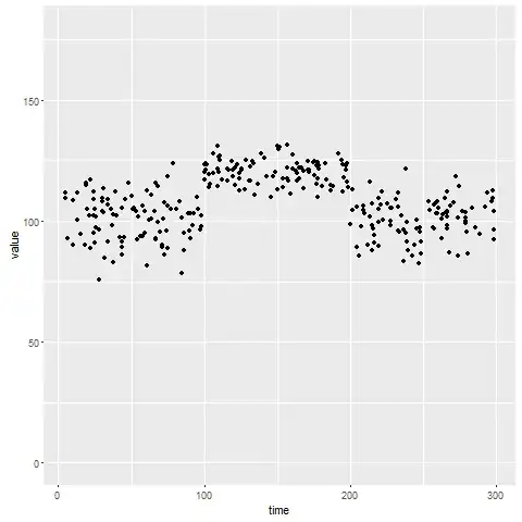
First we are gonna generate some data (i'm using dplyr and ggplot2 packages - but you can handle data with other means):

mydata <- dplyr::bind_rows(
    data.frame(time = sample(1:100, size = datasize, replace = T),
               value = rnorm(datasize, mean = 100, sd = 10),
               group = 1),
    data.frame(time = sample(100:200, size = datasize, replace = T),
               value = rnorm(datasize, mean = 120, sd = 5),
               group = 2),
    data.frame(time = sample(200:300, size = datasize, replace = T),
               value = rnorm(datasize, mean = 100, sd = 8),
               group = 3))

ggplot(mydata, aes(x = time, y = value)) +
  geom_point() +
  ylim(c(0, 180)) 

---

Static approach (and unsupervised)

So you "see" clusters of points that are slightly shifted. That is actually independent of "time" - just consider time and value "static" random variables. What you can do is simple clustering. In order to also get some parameter estimates we can consider the data value as a mixture of Gaussians and use the EM Algorithm (package mixtools required):

mixn <- mixtools::normalmixEM(mydata$value, k = 3, maxit = 10^4)
mixn[c("mu", "sigma")]

$mu
[1] 100.8723 104.5275 120.0161

$sigma
[1] 9.5199389 0.9243747 5.1829086

The means are more or less captures accurately, but the sigmas not so much. Anyhow, your mixture would look like this:

You would then, for every point, compute its likelihood belonging to either distribution - and choose a class with the maximal likelihood.

Furthermore, we can compute more precise clusters using value and time variable togther - again from a static point of view.

mixmvn <- mixtools::mvnormalmixEM(as.matrix(mydata[c("time", "value")]), k = 3)

Although the result seems nice, you need to deal with covariance matrices for interpretation.

---

Dynamic approach (and supervised)

What you may looking for are Hidden Markov Models. In their basic version they model discrete states with discrete observations. They can be extended to continous observations. (Btw: continous state and constinous obeservations are related to the topic of Kalman-filters).

To estimate the parameters we can use package RHmm which atm can only be installed from achive RHmm archive by R CMD INSTALL R_Hmm_2.0.3.tar.gz.

# we need to order the values by time
orderedValues <- (mydata %>% dplyr::arrange(time))$value

hmm <- RHmm::HMMFit(obs = orderedValues, nStates = 3, dis = "NORMAL", list(iter = 1000, nInit = 100), asymptCov = F)

The results are very nice:

> hmm$HMM$distribution

Model:
3 states HMM with univariate gaussian distributions

Distribution parameters:
             mean      var
State 1 120.28424 24.27617
State 2  97.56794 72.53311
State 3 106.79554 31.86263
> sqrt(hmm$HMM$distribution$var) # sigma
[1] 4.927085 8.516637 5.644699

The means as well as sigmas are estimated more or less correctly. We can use predict for new samples in order to assign a state if we want.

All these methods has a distadvantage, however. They all need a fist estimate of number states.

If you are only interested in "change" in dynamic (and have a lot of data), a Hebb's rule may be your friend. Afaik Hebb's rule get accustomed to your data and you will see a spike if the sequential input changes "dramatically".

Any thoughts ?

Answer 2

First you can verify that the process is heteroscedastic: https://en.wikipedia.org/wiki/Heteroscedasticity

Or that there is a moving average: https://en.wikipedia.org/wiki/Moving_average

If there is, then it is case depending how to proceed as Arun Jose has said. When designing algorithms you might want to look into window functions or kernels. Kernels are better and more rigor, but mathematically harder to understand, and thus to implement.

Answer 3

Yes, you can do it!

What you're looking for is machine learning, a set of test data and a good enough algorithm.

Machine learning is a method of data analysis that automates analytical model building. Using algorithms that iteratively learn from data, machine learning allows computers to find hidden insights without being explicitly programmed where to look. source

If you have some programming expertise then I recommend you start here. These tutorials are very easy to follow along and you'll get a basic idea about ML itself.