The real-life problem
Assume I put a spherical roast with initially constant temperature of start_temp=25 (°C) into an oven with oven_temp=80. A meat thermometer is inserted at the core.
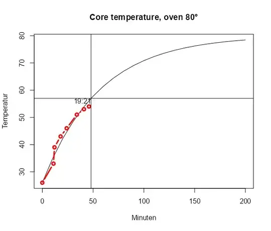
At what time will the roast be ready, i.e. at target_temp=57?
No discussion about rare or well-done, please, this is serious science. The assumption of a constant initial temperature in the sphere is a bit frivolous because the roast is usually fried in a pan before inserting it into the oven, but let's keep this for further research.
The theory
As of the Fourier expansion of heat transfer, page 43, this can be approximated by an exponential curve.
tfun = function(time,  th) {
  start_temp + (oven_temp - start_temp) * (1 - exp(-time / th))
}
Using more terms of the Fourier series expansion is easily possible, but does not contribute to the fit quality.
We do not care that estimates of thermal conductivity and radius could give us an initial approximation, because the fit works reasonably and gives a good estimate of the time when the family has to stop playing Flight Simulator. See the R-program below.
The extended real-life problem
The family suddenly request that the temperature should be lowered to 60 degrees for a more even meat texture or more time to finish the landing. So at t= 30 minutes, we switch the oven from 80° to 60°; assume it cools immediately.
The extended theory
This requires me to solve the inhomogeneous equation with a step function at the boundary, with all the nasty singularities at the center (Thibault et al.). I failed to get it to work with simulated data.
Does anyone have an idea for a simplified fit piecewise function to use? The final code will be in c# (on Android), but Python or R are fine.
The wild extension:
There are Bluetooth-devices with two sensors, so one could be inside the meat, the other in the oven. This would mean that oven temperature and roast core temperature are given in a minute-grid.
# At what time can we serve the roast?
https://pnp.mathematik.uni-stuttgart.de/igt/eiserm/lehre/HM3/HM3-S-1x2.pdf
page 43
d = data.frame(
  time = c("18:33", "18:44", "18:45", "18:51", "18:57", "19:07", "19:14", "19:19"),
  temp = c(26, 33, 39, 43, 46, 51, 53,54 )
)
d$tmin = as.numeric((strptime(d$time, "%H:%M") - strptime(d$time[1], "%H:%M")) /
                      60)
oven_temp = 80 # Oven temperature, constant
target_temp = 57 # Requested core temperature
start_temp = d$temp[1]
tfun = function(time,  th) {
  start_temp + (oven_temp - start_temp) * (1 - exp(-time / th))
}
I am using a nonlinear fit here. Fitting linear regression
to log-data works fine, but would not be generalizable
to more complex functions.
coef(nls(temp ~ tfun(tmin, th), start = list(th = 50), data = d))
time = seq(0, 200, by = 10)
th_1 = coef(nls(temp ~ tfun(tmin, th), start = list(th = 90), data = d))
plot(
  time,
  tfun(time, th_1),
  type = "l",
  ylab = "Temperatur",
  xlab = "Minuten",
  main = paste0("Core temperature, oven ", oven_temp, "°")
)
lines(d$tmin, d$temp,col = "red",lwd = 3, type = "b")
abline(h = target_temp)
tfun_target = function(time, th) {
  tfun(time, th) - target_temp
}
target_minute = as.integer(uniroot(tfun_target, c(0, 300), th = th_1)$root)
abline(v = target_minute)
text(target_minute,
     target_temp,
     adj = c(1, 1),
     format(strptime(d$time[1], "%H:%M") + target_minute * 60, "%H:%M"))
