Optimal transport warping implementation in Matlab

Question

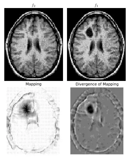
I am implementing the paper "Optimal Mass Transport for Registration and Warping", my goal being to put it online as I just cannot find any eulerian mass transportation code online and this would be interesting at least for the research community in image processing.

The paper can be summarized as follows :
- find an initial map $u$ using 1D histogram matchings along the x and y coordinates
- solve for the fixed point of $u_t = \frac{1}{\mu_0} Du \nabla^\perp\triangle^{-1}div(u^\perp)$ , where $u^\perp$ stands for a 90 degrees counter clockwise rotation, $\triangle^{-1}$ for the solution of the poisson equation with Dirichlet boundary conditions (=0), and $Du$ is the determinant of the Jacobian matrix.
- stability is guaranteed for a timestep $dt<\min|\frac{1}{\mu_0}\nabla^\perp\triangle^{-1}div(u^\perp)|$

For numerical simulations (performed on a regular grid), they indicate using matlab's poicalc for solving the poisson equation, they use centered finite differences for spatial derivatives, except for $Du$ which is computed using an upwind scheme.

Using my code, the energy functional and curl of the mapping are properly decreasing for a couple iterations (from a few tens to a few thousands depending on the time step). But after that, the simulation explodes : the energy increases to reach a NAN in very few iterations. I tried several orders for the differentiations and integrations (a higher order replacement to cumptrapz can be found here), and different interpolation schemes, but I always get the same issue (even on very smooth images, non-zero everywhere etc.).
Anyone would be interested in looking at the code and/or the theoretical problem I am facing ? The code is rather short.

• Code with debugging functions

  • registration function
  • test code provided you have two images of the same size to register

• Just the necessary function without test stuffs (< 100 lines)

Please replace gradient2() at the end by gradient(). This was a higher order gradient but doesn't solve things either.

I am only interested in the optimal transport part of the paper for now, not the additional regularization term.

Thanks !

Answer 1

My good friend Pascal made this a few years ago (it's almost in Matlab):

#! /usr/bin/env python

#from scipy.interpolate import interpolate
from pylab import *
from numpy import *


def GaussianFilter(sigma,f):
    """Apply Gaussian filter to an image"""
    if sigma > 0:
        n = ceil(4*sigma)
        g = exp(-arange(-n,n+1)**2/(2*sigma**2))
        g = g/g.sum()

        fg = zeros(f.shape)

        for i in range(f.shape[0]):
            fg[i,:] = convolve(f[i,:],g,'same')
        for i in range(f.shape[1]):
            fg[:,i] = convolve(fg[:,i],g,'same')
    else:
        fg = f

    return fg


def clamp(x,xmin,xmax):
    """Clamp values between xmin and xmax"""
    return minimum(maximum(x,xmin),xmax)


def myinterp(f,xi,yi):
    """My bilinear interpolator (scipy's has a segfault)"""
    M,N = f.shape
    ix0 = clamp(floor(xi),0,N-2).astype(int)
    iy0 = clamp(floor(yi),0,M-2).astype(int)
    wx = xi - ix0
    wy = yi - iy0
    return ( (1-wy)*((1-wx)*f[iy0,ix0] + wx*f[iy0,ix0+1]) +
        wy*((1-wx)*f[iy0+1,ix0] + wx*f[iy0+1,ix0+1]) )


def mkwarp(f1,f2,sigma,phi,showplot=0):
    """Image warping by solving the Monge-Kantorovich problem"""
    M,N = f1.shape[:2]

    alpha = 1
    f1 = GaussianFilter(sigma,f1)
    f2 = GaussianFilter(sigma,f2)

    # Shift indices for going from vertices to cell centers
    iUv = arange(M)             # Up
    iDv = arange(1,M+1)         # Down
    iLv = arange(N)             # Left
    iRv = arange(1,N+1)         # Right
    # Shift indices for cell centers (to cell centers)
    iUc = r_[0,arange(M-1)]
    iDc = r_[arange(1,M),M-1]
    iLc = r_[0,arange(N-1)]
    iRc = r_[arange(1,N),N-1]
    # Shifts for going from centers to vertices
    iUi = r_[0,arange(M)]
    iDi = r_[arange(M),M-1]
    iLi = r_[0,arange(N)]
    iRi = r_[arange(N),N-1]


    ### The main gradient descent loop ###      
    for iter in range(0,30):
        ### Approximate derivatives ###
        # Compute gradient phix and phiy at pixel centers.  Array phi has values
        # at the pixel vertices.
        phix = (phi[iUv,:][:,iRv] - phi[iUv,:][:,iLv] + 
            phi[iDv,:][:,iRv] - phi[iDv,:][:,iLv])/2
        phiy = (phi[iDv,:][:,iLv] - phi[iUv,:][:,iLv] + 
            phi[iDv,:][:,iRv] - phi[iUv,:][:,iRv])/2
        # Compute second derivatives at pixel centers using central differences.
        phixx = (phix[:,iRc] - phix[:,iLc])/2
        phixy = (phix[iDc,:] - phix[iUc,:])/2
        phiyy = (phiy[iDc,:] - phiy[iUc,:])/2
        # Hessian determinant
        detD2 = phixx*phiyy - phixy*phixy

        # Interpolate f2 at (phix,phiy) with bilinear interpolation
        f2gphi = myinterp(f2,phix,phiy)

        ### Update phi ###
        # Compute M'(phi) at pixel centers
        dM = alpha*(f1 - f2gphi*detD2)
        # Interpolate to pixel vertices
        phi = phi - (dM[iUi,:][:,iLi] + 
            dM[iDi,:][:,iLi] + 
            dM[iUi,:][:,iRi] + 
            dM[iDi,:][:,iRi])/4


    ### Plot stuff ###      
    if showplot:
        pad = 2
        x,y = meshgrid(arange(N),arange(M))
        x = x[pad:-pad,:][:,pad:-pad]
        y = y[pad:-pad,:][:,pad:-pad]
        phix = phix[pad:-pad,:][:,pad:-pad]
        phiy = phiy[pad:-pad,:][:,pad:-pad]

        # Vector plot of the mapping
        subplot(1,2,1)
        quiver(x,y,flipud(phix-x),-flipud(phiy-y))
        axis('image')
        axis('off')
        title('Mapping')

        # Grayscale plot of mapping divergence
        subplot(1,2,2)  
        divs = phixx + phiyy # Divergence of mapping s(x)
        imshow(divs[pad:-pad,pad:-pad],cmap=cm.gray)
        axis('off')
        title('Divergence of Mapping')
        show()

    return phi


if __name__ == "__main__":  # Demo
    from pylab import *
    from numpy import * 

    f1 = imread('brain-tumor.png')
    f2 = imread('brain-healthy.png')
    f1 = f1[:,:,1]
    f2 = f2[:,:,1]

    # Initialize phi as the identity map
    M,N = f1.shape
    n,m = meshgrid(arange(N+1),arange(M+1))
    phi = ((m-0.5)**2 + (n-0.5)**2)/2

    sigma = 3
    phi = mkwarp(f1,f2,sigma,phi)
    phi = mkwarp(f1,f2,sigma/2,phi,1)
#   phi = mkwarp(f1,f2,sigma/4,phi,1)

The gradient descent approach is explained here: people.clarkson.edu/~ebollt/Papers/quadcost.pdf