Duality of these two 'flavours'
The non-existance of value assignments that are independent of the context of measurements is related to the non-existance of noncontextual ontological models for the statistics generated because the value assignments that you have described $\nu: \mathcal{B}(\mathcal{H})_{sa} \to \mathbb{R}$ would serve as an ontic state as $\nu \in \Lambda$ with $\Lambda$ the full set of ontological explanations of the experiment satisfying that $\nu(A) = f_A(\nu)$ and $f_A:\Lambda \to \mathbb{R}$ is a function over the ontic state-space towards the pre-determined values that a self-adjoint observable $A$ may have. There is a very nice discussion (mathematically rigorous and historically relevant) in this Master Dissertation. The deterministic value assignments represent the complete states of knowledge while any statistics a system present should then assign a probability distribution over all possible value assignments in general. Let then the set of all possible valuations that are classical and compatible with an experimental scenario (they don't always exist) be named $\mathcal{V} \equiv \Lambda$ we have that for projections $P_a$ a Kochen-Specker noncontextual model is of the form
$$\text{Tr}(\rho P_a) = \sum_{\nu \in \mathcal{V}} p_\nu \nu(P_a)$$
where normally in some formalisms and works it is stressed that $p_\nu \equiv p(\nu\vert \rho)$, while the relevant point is really that $p_\nu \in [0,1]$ for all $\nu$ and $\sum_{\nu \in \mathcal{V}}p_\nu =1$. This description is beautifully described in this recent paper, Chapter II, other chapters are technical results about something else.
The important thing is that this description in terms of a realist model is totally equivalent to existing a global distribution for the measurement scenario that is also nondisturbing (or equivalently nonsignaling in Bell scenarios). This is the content of the Fine-Abramsky-Brandenburger theorem proved in Ref4, Ref5, Ref6 and more recently a beautiful proof presented for continuous case in Ref7.
FAB Result Informally Stated: Considering any measurement scenario (to be properly defined in the references) the following are equivalent: (i) data-tables can be explained by noncontextual hidden-variable models (ii) data-tables allow for a global distribution explaining them via marginals over contexts.
The references have very formal formulations of this result. As well as proofs.
Peres-Mermin in terms of Inequalities
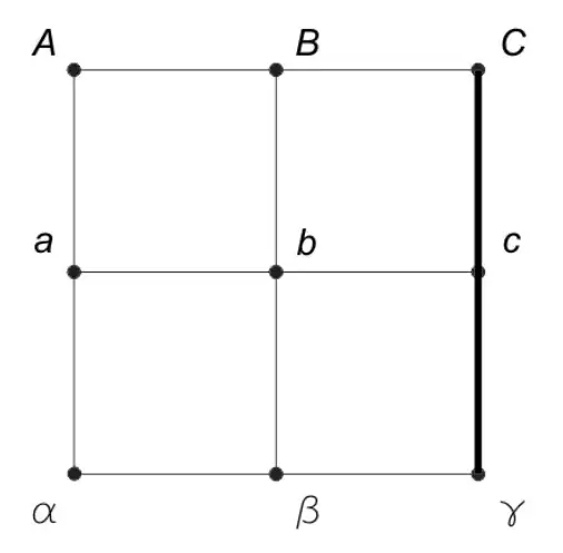
The PM square generates an inequality that is particularly tricky and highly nontrivial so this is the reason why it is so complicated to understand how it can relate to operational distributions. However the problem is not really on the formulation of the probabilities, and in writing the inequality. The problem is to be careful with the experimental implementations. If you simply follow the beggining of this review on quantum contextuality, the notation for the PM square is the following: Consider the following scenario, you have nine dichotomic measurements $\{A,B,C,a,b,c,\alpha,\beta,\gamma\}$ and you have they can be put in a way that they form a table with each row and each columns forming a measurement context.
$$\left[\begin{matrix} A & B & C \\ a & b & c \\ \alpha & \beta & \gamma \end{matrix}\right]$$
Given that we know that the measurements are dichotomic, and that what we are really interested is in the compatibility relations of those procedures, we can encode this information in a graph (this is way we have graph-approaches to contextuality, because all the compatibility information relevant for contextuality of measurement procedures can be encoded in graph-theoretic structures). The picture below has the graph, and each row/column line depicts a (hyper)edge defining the context of the measurement procedures.
Since we have dichotomic measurements with outcomes in $\{+1,-1\}$ each conditional probability for the contexts jointly measured can be written as $$\langle C \rangle = p(C = +1) - p(C = -1)$$ for each context $C$ in the set of all contexts $\mathcal{C} = \{ABC,abc,\alpha\beta\gamma,Aa\alpha,Bb\beta,Cc\gamma\}$ and therefore one can find the following operational inequality,
$$\langle ABC \rangle + \langle abc \rangle + \langle \alpha\beta\gamma \rangle + \langle Aa\alpha \rangle + \langle Bb\beta \rangle - \langle Cc\gamma \rangle \leq 4$$
And the quantum realization that is very well known,
$$\left[\begin{matrix} A & B & C \\ a & b & c \\ \alpha & \beta & \gamma \end{matrix}\right] = \left[\begin{matrix} Z\otimes I & I\otimes Z & Z\otimes Z \\ I\otimes X & X\otimes I & X\otimes X \\ Z\otimes X & X\otimes Z & Y\otimes Y \end{matrix}\right]$$
Reaches the value $6$. Note that $p(C=+1)$ encodes the probability distributions $p(C = +1) = \sum_{a_1a_2a_3=+1} p(a_1a_2a_3\vert x_1x_2x_3)$ and therefore the inequality discussed is in the form you wanted; the sum is over all products of outcomes that are equal to $+1$ such as $a_1=-1,a_2=-1,a_3=+1$. Note also that this state-independent proof of the KS theorem is also the largest possible value the inequality can take, which is associated to the fact these proofs are also strongly contextual empirical models.
To obtain the inequality you may consider all deterministic valuations that are vertices of the convex polytope of classical assignments. This vector will be something like $(v(A),v(B),\dots, v(\gamma), v(ABC), \dots, v(\alpha\beta\gamma))$ and there will be $2^9$ possible vectors of this form satisfying the constraint that $v(ABC) = v(A)v(B)v(C)$. With the $V$-representation of this polytope you can find the $H$-representation using standard convex optimization techniques. Here is a program that does that. Important disclaimer: there might be more terms in the construction of these vectors, like terms of the form $v(Aa)$, I am not sure since I haven't do the calculations myself for this particular case, but I think you got the idea, in case I learn properly about this I shall edit this question. What is relevant nevertheless is that the values $v(Aa\alpha) = v(A)v(a)v(\alpha)$ and $v(ABC) = v(A)v(B)v(C)$ with the same value $v(A)$ supposed to be independent on the measuring context considered (measurement noncontextuality, if we would have measurement contextuality then $v(A)$ would need a new label $C$ saying the context of the value assignment $v(A\vert C)$). The original paper that proposed the inequality just presented is the following one: Ref3!
Note also how this parallels entirely the derivation of the full set of Bell inequalities. Arxiv version here.
Discussion of this inequality: One must be very careful with experimentally testing this inequality. The first discussion on $3$ common misleading things in the review paper mentioned the importance that the experiment must attest the contexts in a specific way as discussed. Moreover, they also address criticism (see pg. 4 after 'A third ...') made elsewhere commenting on the differences between the Kochen-Specker formalism and the generalized noncontextuality (or Spekkens) formalism. In these papers Ref1 Ref2, on Appendix D and Appendix III.A respectively, they argue that all vertex valuations would be logically impossible to begin with, and therefore are not representing anything new in terms of non-existing of non-contextual models. The review paper discusses this issue. But note that the matter of noncontextuality inequalities is complicated, to say the least.
