The standard methodology for a single "variable" (such
as price-to-book) is this: 1. Sort the stocks in the
cross-section at a specific point in time by that
variable. 2. Compare the subsequent returns of stocks
that have a high value of the variable, with returns of
stocks that a low value of the variable. To do this
comparison, you'd take the difference between the
returns of high-value-of-variable stocks, and returns
of low-value-of-variable stocks. This, in turn,
corresponds naturally to being long one portfolio of
stocks (high-value-of-variable), and being short another portfolio
(low-value-of-variable).
Statistically, if there is a monotone relation between
the variable and subsequent stock returns, the spread
in returns will be greater if you look at long/short
portfolios, and so the power of your tests increases.
(That is, the relation between variable and return is
easier to spot.)
That being said, as an investor, you will want to
analyze to what extent long and short positions have
contributed to total return. For instance, if you find
that the short portfolio was responsible for a substantial
portion of total return, then not implementing it
would mean the strategy becomes less attractive. (But
of course, it need not be an actual short position. As
pointed out in the comment by nbbo2, it might be a
negative active weight relative to a benchmark.)
Kenneth French publishes several datasets that show the
returns of the original sort portfolios, i.e. not just the
long--short aggregate returns. For instance, momentum
(i.e., the variable you sort on is 1-year return). The
figure below shows the total returns of 10 momentum
portfolios since 1970, with 10 being the high-momentum
portfolio and 1 the low-momentum portfolio (the lighter
the grey, the higher the momentum). In blue, I have
added the market return.
library("NMOF")
library("zoo")
library("PMwR")
P <- French(dest.dir = tempdir(),
            dataset = "10_Portfolios_Prior_12_2_CSV.zip",
            weighting = "value",
            price.series = TRUE, na.rm = TRUE)
P <- window(zoo(P, as.Date(row.names(P))),
            start = as.Date("1969-12-31"))
M <- French(tempdir(), dataset = "market",
            price.series = TRUE, na.rm = TRUE)
M <- window(zoo(M, as.Date(row.names(M))),
            start = as.Date("1969-12-31"))
greys <- grey(seq(.1, .6, length.out = ncol(P)))
par(las = 1, mar = c(3,5,1,2))
plot(P <- scale1(P, level = 100),
     plot.type = "single", log = "y",
     xlab = "", ylab = "Performance",
     col = greys)
lines(scale1(M, level = 100), col = "blue", lwd = 2)
par(xpd=TRUE)
text(x = max(index(M)), y = c(coredata(tail(P, 1))),
     labels = 1:10, pos = 4, col = greys)
par(xpd=FALSE)
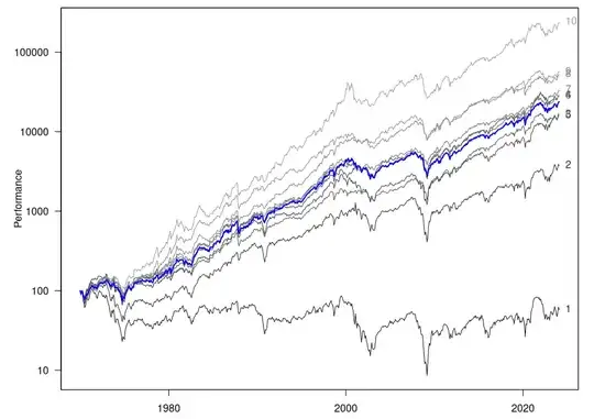
As you can see, the
high-momentum portfolio beats the market, while the
low-momentum portfolio underperforms. The headline
"momentum-return" number aggregates both sources of
outperformance.
