7

I'm building a manufacturing line optimization model. Part of the model is (lightly) penalizing running the line on the weekend. With time in minutes and t=0 representing 12:00:01 am Monday, the weekend begins at t=7200 (end of 5 days, start of Saturday) and ends at t=10080 (end of 7 days, start of Monday). I have decision variables around when a manufacturing run starts and ends. I'd like to make a decision variable to quantify how much of the manufacturing run occurs on the weekend (not just if it does or not - I want to know the magnitude.)

So for example:

run start time = 7000, run end time = 7199 : 0 overlap (weekend minutes)

run start time = 7000, run end time = 7300 : 100 overlap

run start time = 8000, run end time = 9000 : 1000 overlap

run start time = 10000, run end time = 11000 : 920 overlap

To clarify, a manufacturing run can overlap the weekend either not at all, partially, or entirely. I'm modeling a monthly or longer time horizon, so I'd repeat the procedure for 4+ weekends.

All the posts I've seen are just to identify if an overlap occurs, not a magnitude.

A.Omidi
  • 8,832
  • 2
  • 13
  • 49
Ralph Asher
  • 763
  • 3
  • 10
  • So the overlap is always with the weekend being at the end - there are no working days after the weekend? – CMichael Mar 31 '22 at 05:19
  • Assume that start[i] and end[i] are the variables for the start and end time for job i, then max(end[i], 7200) - max(start[i], 7200) should give you the time of the job that is executed at the weekend. This assumes that jobs do terminate before Monday (as suggested by @CMichael). – Daniel Junglas Mar 31 '22 at 05:23
  • 1
    By the way MIP is not the best option for scheduling. With CPOptimizer within CPLEX you may use the function overlapLength – Alex Fleischer Mar 31 '22 at 06:04
  • @DanielJunglas Do you mean $\min{\mbox{end}_i,10800}-\max{\mbox{start}_i,7200}$ ? Note that this is not linear though. – Kuifje Mar 31 '22 at 10:44
  • No, jobs do not have to finish before Monday. So a job that starts Thursday, then runs through Tuesday afternoon, is possible and the overlap is the whole two days. @AlexFleischer it's not a CP, I have an objective function associated with what's produced on the line and it's not possible to produce enough to satisfy demand in the time horizon. So I need to use MIP instead of a sat solver – Ralph Asher Mar 31 '22 at 12:10
  • @CMichael This is on a monthly horizon, four weekends - so yes, working days after the (first three) weekends – Ralph Asher Mar 31 '22 at 13:17
  • 1
    You can optimize a linear objective function using using CPOptimizer. – prubin Mar 31 '22 at 15:20
  • @RalphAsher, is the answer by Kuifje what you want? If not, why you do not decompose the planning horizon into two sections, first on the daily shift and the second on the weekend shift, and declaring two decision variables to capture production runs and their corresponding penalties? – A.Omidi Apr 01 '22 at 16:41

1 Answers1

9

If you just want to know the magnitude of the overlap after optimization, then you can use the following formula for a given job $i$, if $\mbox{start}_i < 10800$: $$\max\{0,\min\{\mbox{end}_i,10800\}-\max\{\mbox{start}_i,7200\}\} \tag{0}$$

If you want to use the overlap in your model as a variable, then you can proceed as follows:

Let $s,e$ denote the start and end time variables, respectively. Let $\ell, u$ denote the start and end times of the weekend, respectively.

Also, let $\delta_1 \in \{0,1\}$ be a binary variable that takes value $1$ if $\ell < s < u$, let $\delta_2 \in \{0,1\}$ be another binary variable that takes value $1$ if $\ell < e < u$, let $\delta_3 \in \{0,1\}$ be another binary variable that takes value $1$ if $e \le \ell$, and let $\delta_4 \in \{0,1\}$ be another binary variable that takes value $1$ if $s \ge u$.

And finally, let $O\in \mathbb{R}^+$ denote the magnitude of the overlap.

You want to model the following:

enter image description here

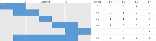
Or in algebraic terms:

\begin{align} \ell < s < u \quad &\Longleftrightarrow \quad \delta_1 \tag{1} \\ \ell < e < u \quad &\Longleftrightarrow \quad \delta_2 \tag{2} \\ e \le \ell \quad &\Longleftrightarrow \quad \delta_3 \tag{3} \\ u \le s \quad &\Longleftrightarrow \quad \delta_4 \tag{4} \\ \delta_1 \wedge \delta_2 \quad &\Longrightarrow \quad O = e-s \tag{5} \\ \delta_1 \wedge \neg \delta_2 \quad &\Longrightarrow \quad O = u-s \tag{6} \\ \neg \delta_1 \wedge \delta_2 \quad &\Longrightarrow \quad O = e-\ell \tag{7} \\ \neg \delta_1 \wedge \neg \delta_2 \wedge (\delta_3 \vee \delta_4) \quad &\Longrightarrow \quad O = 0 \tag{8} \\ \neg \delta_1 \wedge \neg \delta_2 \wedge \neg \delta_3 \wedge \neg \delta_4 \quad &\Longrightarrow \quad O = u - \ell \tag{9} \end{align}

For $(1)$, use the following big M constraints: \begin{align} \ell + \epsilon -M(1-\delta_1) \le s \le u - \epsilon + M(1-\delta_1) \tag{1a} \\ u -M(1-y_1) \le s \le \ell + M(1-y_2) \tag{1b} \\ \delta_1+y_1 +y_2 = 1 \tag{1c} \\ \delta_1,y_1, y_2 \in \{0,1\} \end{align} For $(2)$, use the following big M constraints: \begin{align} \ell + \epsilon-M(1-\delta_2) \le e \le u -\epsilon + M(1-\delta_2) \tag{2a}\\ u -M(1-y_3) \le e \le \ell + M(1-y_4) \tag{2b} \\ \delta_2+y_3 +y_4 = 1 \tag{2c} \\ \delta_2,y_3, y_4 \in \{0,1\} \end{align} For $(3)$, use the following big M constraints: $$ \ell + \epsilon -M\delta_3 \le e \le \ell +M(1-\delta_3) \tag{3a}\\ \delta_3 \in \{0,1\} $$ For $(4)$, use the following big M constraints: $$ u - M(1-\delta_4)\le s \le u - \epsilon + M \delta_4 \tag{4a} \\ \delta_4 \in \{0,1\} $$

For $(5)$, use the following big M constraints: $$ e - s - M (2-\delta_1 - \delta_2) \le O \le e - s + M (2-\delta_1 - \delta_2) \tag{5a} \\ \delta_1,\delta_2 \in \{0,1\} $$

For $(6)$, use the following big M constraints: $$ u - s - M (1-\delta_1 + \delta_2) \le O \le u - s + M (1-\delta_1 + \delta_2) \tag{6a}\\ \delta_1,\delta_2 \in \{0,1\} $$

For $(7)$, use the following big M constraints: $$ e - \ell - M (1-\delta_2 + \delta_1) \le O \le e - \ell + M (1-\delta_2 + \delta_1) \tag{7a}\\ \delta_1,\delta_2 \in \{0,1\} $$

For $(8)$, use the following big M constraints: \begin{align} 0 - M (\delta_1 + \delta_2 + 1- \delta_3) \le O \le 0 + M (\delta_1 + \delta_2 + 1-\delta_3 ) \tag{8a} \\ 0 - M (\delta_1 + \delta_2 + 1 -\delta_4) \le O \le 0 + M (\delta_1 + \delta_2 + 1-\delta_4 ) \tag{8b} \\ \delta_1,\delta_2,\delta_3,\delta_4 \in \{0,1\} \end{align} For $(9)$, use the following big M constraints: $$ u - \ell - M (\delta_1 + \delta_2 + \delta_3 + \delta_4) \le O \le u - \ell + M (\delta_1 + \delta_2 + \delta_3 + \delta_4 ) \tag{9a}\\ \delta_1,\delta_2,\delta_3,\delta_4 \in \{0,1\} $$

Note also that by definition $\delta_1 \; \Longrightarrow \; \neg \delta_3$, $\delta_1 \; \Longrightarrow \; \neg \delta_4$, $\delta_2 \; \Longrightarrow \; \neg \delta_3$, $\delta_2 \; \Longrightarrow \; \neg \delta_4$: $$ \delta_1 \le 1- \delta_3 \\ \delta_1 \le 1- \delta_4 \\ \delta_2 \le 1- \delta_3 \\ \delta_2 \le 1- \delta_4 \\ $$


Note : Ideally, distinguish the different big $Ms$. Also, I would not be surprised if the above constraints could be simplified. In particular, I am not 100% sure if the double implication is required in constraints $(1)-(4)$.


Addendum

OP uses a formulation which linearizes equation $(0)$, without any binary variables. OP minimizes $O$ subject to \begin{align} O &\ge u - \ell - \alpha - \beta \\ \alpha &\ge s- \ell \\ \beta &\ge u -e \\ \alpha, \beta, O &\ge 0 \\ \end{align} which is equivalent to \begin{align} O &\ge (u - \max\{u -e, 0\}) - (\ell + \max\{s- \ell, 0\})\\ O &\ge 0 \end{align} or \begin{align} O &\ge \min\{u,e\} - \max\{s,\ell\}\\ O &\ge 0 \end{align}

which yields $$ O = \max\{0,\min\{u,e\} - \max\{s,\ell\}\} $$

Note however that this works because we are minimizing.

Kuifje
  • 13,324
  • 1
  • 23
  • 56
  • Thanks. Yes I do want to use the magnitude as a decision variable, not just evaluate in postprocessing the results. I came up with an approach that didn't use binary variables, but it was dependent upon including some penalties in the objective function - something I am a little weary about initially. – Ralph Asher Mar 31 '22 at 12:17
  • 1
    I think it would be interesting if you shared your formulation with penalties. – Kuifje Mar 31 '22 at 12:27
  • Define decision variables: activity_start, activity_end , Define scalars weekend_start, weekend_end. Define continuous variables alpha,beta, overlap_length. All lower-bounded at zero. Define constraints alpha >= activity_start - weekend_start , beta >= weekend_end - activity_end. overlap_length >= weekend_end - weekend_start - alpha - beta . Ideally, alpha and beta will be treated as equality constraints iff >= 0, and the last constraint would be an equality constraint also. – Ralph Asher Mar 31 '22 at 12:48
  • This formulation works in all possible cases of overlap / nonoverlap, but only if you can appropriately shape the objective function to make alpha, beta, and overlap_length to be as low as possible within the constraints. – Ralph Asher Mar 31 '22 at 12:54
  • https://github.com/datadrivensupplychain/teaching_bits/blob/main/identify_duration_inside_window_vignette.r R script – Ralph Asher Mar 31 '22 at 12:57
  • Your formulation seems great ! I suppose you have some other terms in the objective function and do not want to add those penalties ? – Kuifje Mar 31 '22 at 13:22
  • 1
    Note also that your formulation is a linearization of the formula $\max{0,\min{\mbox{end}_i,10800}-\max{\mbox{start}_i,7200}}$. – Kuifje Mar 31 '22 at 13:40
  • @Kufje yes, my objective function is to maximize the total output of the line over the monthly horizon (including four weekends). I want to be able to penalize production on the weekend (overlap_length * pounds per minute) in the objective function, to guide the solver to a solution that only uses the weekdays. But that requires me to be very careful about how I penalize overlap_length, alpha, and beta to get their values to equal the minimums without messing up the real, business objective. And yes, I initially just made the formula you listed, then worked out a linearization – Ralph Asher Mar 31 '22 at 14:22