The earliest forms of the extended Euclidean algorithm are ancient, dating back to 5th-6th century A.D. work of Aryabhata - who described the Kuttaka ("pulverizer") algorithm for the more general problem of solving linear Diophantine equations $ ax + by = c$. It was independently rediscovered numerous times since, e.g. by Bachet in 1621, and Fermat and Wallis, and by Euler circa 1731.
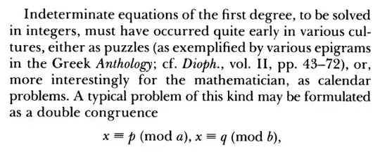
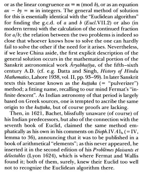
Weil discusses this briefly in his book Number Theory: An Approach through History from Hammurapi to Legendre, excerpted below (from pp. 6-7)
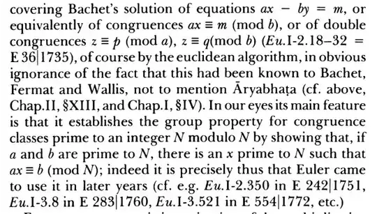
 Euler's rediscovery is mentioned on pp. 176-77:

It deserves to be more widely known that the algorithm is simpler to execute (and remember) if you are already familiar row-operations such as in Gaussian elimination / triangularization in linear algebra. See this MSE answer for a presentation from that viewpoint. This method eliminates the notoriously error-prone back-substitution in the more common presentation of the algorithm. Below is a worked example done this way, computing $\, \gcd(141,19),\, $ shown firstly in full equational form, and secondly in more concise tabular form.
$$\rm\begin{eqnarray}[\![1]\!]\!\quad \color{#C00}{141}\!\ &=&\,\ \ \ 1&\cdot& 141\, +\ 0&\cdot& 19 \\
[\![2]\!]\quad\ \color{#C00}{19}\ &=&\,\ \ \ 0&\cdot& 141\, +\ 1&\cdot& 19 \\
\color{#940}{[\![1]\!]-7\,[\![2]\!]}\, \rightarrow\, [\![3]\!]\quad\ \ \ \color{#C00}{ 8}\ &=&\,\ \ \ 1&\cdot& 141\, -\ 7&\cdot& 19 \\
\color{#940}{[\![2]\!]-2\,[\![3]\!]}\,\rightarrow\,[\![4]\!]\quad\ \ \ \color{#C00}{3}\ &=&\, {-}2&\cdot& 141\, + 15&\cdot& 19 \\
\color{#940}{[\![3]\!]-3\,[\![4]\!]}\,\rightarrow\,[\![5]\!]\quad \color{#C00}{{-}1}\ &=&\,\ \ \ 7&\cdot& 141\, -\color{}{ 52}&\cdot& \color{}{19} \end{eqnarray}\qquad\qquad\qquad$$
$$\rm\begin{eqnarray} &&[\![1]\!]\quad \color{#C00}{141} &\ \ \ 1 &\quad\ \ 0 \\
&&[\![2]\!]\quad\ \color{#C00}{19} &\ \ \ 0 &\quad \ \ 1 \\
\color{#940}{[\![1]\!]-7\,[\![2]\!]}\,\rightarrow\,&&[\![3]\!]\quad\ \ \ \color{#C00}{ 8} &\ \ \ 1 &\ -7\\
\color{#940}{[\![2]\!]-2\,[\![3]\!]}\,\rightarrow\,&&[\![4]\!]\quad\ \ \ \color{#C00}{3} & -2 &\ \ \ \, 15 \\
\color{#940}{[\![3]\!]-3\,[\![4]\!]}\,\rightarrow\,&&[\![5]\!]\quad \color{#C00}{{-}1} &\ \ \ 7 & \, \color{}{{-}52} \end{eqnarray}\qquad\qquad\qquad\qquad\qquad\quad\ $$
One can optimize even further (e.g. see the fractional form below). It would be interesting to know who first presented the algorithm from this viewpoint. Likely it as at least a few centuries old.
It would take immense effort to write a good history of the extended Euclidean algorithm and related ideas, since it occurs in many different guises throughout mathematics, e.g. search on the following keywords: Hermite / Smith normal form,
invariant factors, lattice basis reduction, continued fractions,
Farey fractions / mediants, Stern-Brocot tree / diatomic sequence.
In fact even in recent times there are useful twists on the algorithm that are discovered, e.g. we can present the algorithm efficiently in fractional form using modular arithmetic, e.g. below I show how we can compute $\,1/117\equiv\color{#c00}{-72} \pmod{337}\ $ this way.
${\rm mod}\ 337\!:\,\ \dfrac{0}{337} \overset{\large\frown}\equiv \dfrac{1}{117} \overset{\large\frown}\equiv \dfrac{-3}{\color{#0a0}{-14}} \overset{\large\frown}\equiv \dfrac{-23}5 \overset{\large\frown}\equiv\color{#c00}{\dfrac{-72} {1}}.\,$ Equivalently, without fractions
$\qquad\quad \begin{array}{rrl}
[\![1]\!]\!:\!\!\!& 337\,x\!\!\!&\equiv\ 0\\
[\![2]\!]\!:\!\!\!& 117\,x\!\!\!&\equiv\ 1\\
[\![1]\!]-3[\![2]\!]=:[\![3]\!]\!:\!\!\!& \color{#0a0}{{-}14}\,x\!\!\!&\equiv -3\\
[\![2]\!]+8[\![3]\!]=:[\![4]\!]\!:\!\!\!& 5\,x\!\!\! &\equiv -23\\
[\![3]\!]+3[\![4]\!]=:[\![5]\!]\!:\!\!\!& \color{#c00}1\, x\!\!\! &\equiv \color{#c00}{-72}
\end{array}$


