Alternatively, you can use the mean of the period, or fit a linear trend and interpolate. These methods use more information than just two years, which has the benefit of accounting for possible idiosyncratic factors in 2012 or 2014, with the cost of perhaps adding idiosyncratic factors from years as far as 2017.
Here is the R code with the three methods (including Alecos's):
# Interpolate between 2012 and 2014
df = data.frame(year = 2010:2017, y = c(22306000,22420000,23010000,NA,25430000,25601000,25267000,23895400))
df$y[is.na(df$y)] = mean(df$y[df$year==2012 | df$year==2014], na.rm=TRUE)

# Replace with mean of period
df = data.frame(year = 2010:2017, y = c(22306000,22420000,23010000,NA,25430000,25601000,25267000,23895400))
df$y[is.na(df$y)] = mean(df$y, na.rm=TRUE)

# Regression interpolation
df = data.frame(year = 2010:2017, y = c(22306000,22420000,23010000,NA,25430000,25601000,25267000,23895400))
fit <- lm(y ~ year, data=df)
df$y[df$year==2013] <- predict(fit, newdata = data.frame(year = 2013))
The results with each method are 24220000, 23989914, and 23753107 respectively. They are different because the series does not follows a linear trend:
# Plot
df = data.frame(year = 2010:2017, y = c(22306000,22420000,23010000,NA,25430000,25601000,25267000,23895400))
plot(x=df$year,df$y, type="l",lwd = 2)
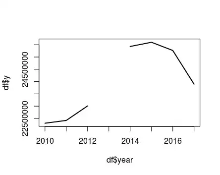
Thus, it seems Aleco's method might be the most appropriate in this case. (It is also possible to fit non-linear trends)
