Noise leakage problem with least square estimation in the frequency-distance domain

Question

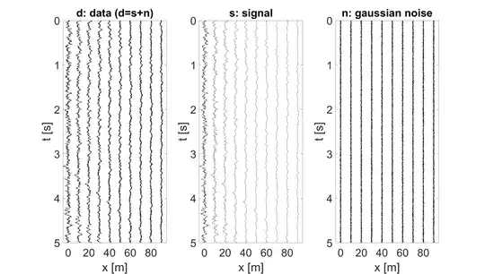
I have data $d$ recorded from an antenna of sensors. These data are composed of a Gaussian noise $n$ and a signal $s$ which I try to estimate. This signal propagates on the antenna with frequency dependent attenuation and velocity. Below is an illustration of such simulated data. We can observe that the signal comes from a source on the left and that the high frequencies are more attenuated.

Assuming that the propagation characteristics of the signal are perfectly known and noting $P$ the vector that propagates the frequency $f$ of the signal on the sensors. It is possible to obtain, frequency by frequency, the least squares estimate of the signal: $\hat{s}(f)=P(P^HP)^{-1}P^Hd(f)$ and then return to the time domain. The result of the estimation applied to the previous data is the following.

The result is quite good except on the first sensor where the noise is estimated. That is to say that there is a leakage of noise in the estimation of the signal. The origin of the phenomenon comes from the strong attenuation of high frequencies. Indeed, the leakage of noise on the first sensor minimizes the residual and, because of the attenuation, does not degrade the one of the following sensors.

My question is how to modify the signal estimation so that I don't have this leakage problem anymore. I have tried to modify the norm and/or regularize the solution but without success.

EDIT: Mathematical model : $d(f)=s(f)+n(f)=s_0(f).P(f)+n(f)$

• $d(f)$: Fourier transform of the data recorded by the $N$ sensors at frequency $f$ (vector of size $N$x$1$)
• $n(f)$: Fourier transform of the Gaussian noise on the $N$ sensors at frequency $f$ (vector of size $N$x$1$)
• $s(f)$: Fourier transform of the signal on the $N$ sensors at frequency $f$ (vector of size $N$x$1$)
• $s_0(f)$: signal generated by the source at the frequency f (complex scalar of size $1$x$1$)
• $P(f)$: Propagator from the source to the position of the sensors at frequency f (vector of size $N$x$1$), s.a. $s(f)=s_0(f).P(f)$

The goal is knowing $d(f)$ and $P(f)$ is it possible to estimate $s(f)$ (without leakage of $n(f)$ in the estimation)?

Below is the MATLAB code used:

N = 10 ; % Number of sensors
M = 1000*5 ; % Number of samples
Delta_x = 10 ; % Distance between sensors
Delta_t = 0.001 ; % Sampling rate
x = (0:N-1).'.*Delta_x ; % positions of sensors
% frequency
Fs = 1/Delta_t ;
dF = Fs/M ;
M_pos = ceil((M+1)/2) ; % Number of "positive" frequencies
f_pos = (0 : M_pos-1)./(Delta_t*M) ;
% Velocity model
vp_f = 25.*(1+sqrt(1+(f_pos./100).^2)) ; % velocity model
% Attenuation model = Gain between sensors at each frequency
%G_f = 0.9.*ones(1,M_pos) ; % Constant
G_f = exp(-sqrt(0.01+(f_pos/100).^2)) ; % High frequencies are more attenuated
% Wavelet generation:
[b,a] = butter(1,10/(Fs/2)) ;
s0 = filter(b,a,randn(M,1)) ;
% Data generation in the frequency-distance domain
FT_s0 = fft(s0) ;
FT_s = zeros(M,N) ;
for ii = 1 : M_pos
    P_f = (G_f(ii).^(0:N-1).').exp(-1i2pi()f_pos(ii)/vp_f(ii)).^x ;
    FT_s(ii,:) = FT_s0(ii).*P_f ;
end
s = ifft(FT_s,'symmetric') ; % back to time domain
% Add noise
n = 0.05.*randn(M,N) ;
d = s+n ;
scale = Delta_x./(2*max(s(:))) ;
figure() ;
subplot(1,3,1) ; w_plot(d, Delta_t, Delta_x, scale) ; title('d: data (d=s+n)','Fontsize',32) ;
subplot(1,3,2) ; w_plot(s, Delta_t, Delta_x, scale) ; title('s: signal','Fontsize',32) ;
subplot(1,3,3) ; w_plot(n, Delta_t, Delta_x, scale) ; title('n: gaussian noise','Fontsize',32) ;
% Estimation
FT_d = fft(d) ;
FT_s_est = zeros(M,N) ;
for ii = 1 : M_pos
    P_f = (G_f(ii).^(0:N-1).').exp(-1i2pi()f_pos(ii)/vp_f(ii)).^x ;
    FT_s_est(ii,:) = (P_f((P_f'P_f)\P_f'))*FT_d(ii,:).' ;
end
s_est = ifft(FT_s_est,'symmetric') ;
figure() ;
subplot(1,3,1) ; w_plot(s, Delta_t, Delta_x, scale) ; title('s: signal','Fontsize',32) ;
subplot(1,3,2) ; w_plot(s_est, Delta_t, Delta_x, scale) ; title('signal estimation','Fontsize',32) ;
subplot(1,3,3) ; w_plot(s - s_est, Delta_t, Delta_x, scale) ; title('difference','Fontsize',32) ;
function w_plot(s, Delta_t, Delta_x, scale)
[M,N] = size(s) ;
x = (0:N-1).Delta_x ;
t = (0:M-1).Delta_t ;
FontSize = 32 ;
plot(scale*s+x,t,'k')
set(gca,'Ydir','reverse');
ylabel('t [s]','FontSize',FontSize) ; xlabel('x [m]','FontSize',FontSize) ;
ax = gca; ax.XAxis.FontSize = FontSize ; ax.YAxis.FontSize = FontSize ;
xlim([x(1)-Delta_x/2 x(end)+Delta_x/2])
end

Answer 1

The model can be rewritten as:

$$ D = P S + N $$

Where $ D, P, N \in \mathcal{C}^{N \times F} $ where $ N $ is the number of sensors and $ F $ is the number of frequencies. The matrix $ S $ is basically $ \operatorname{Diag}\left( \boldsymbol{s}_{0} \right) $ where $ \operatorname{Diag} $ yields a diagonal matrix from a vector.

The least squares solution for $ S $ is given by:

$$ \hat{S} = {\left( {P}^{H} P \right)}^{-1} {P}^{H} D $$

Yet, this won't generate a diagonal matrix.
The optimization problem we're after is:

$$ \begin{align} \arg \min_{S} \quad & {\left\| P S - D \right\|}_{F}^{2} \\ \text{subject to} \quad & \begin{aligned} S & \in \mathcal{D}^{F} = \left\{ D \in \mathbb{C}^{F \times S} \mid {D}_{ij} = \begin{cases} \boldsymbol{d}_{i} & \text{ if } i = j \\ 0 & \text{ if } i \neq j \end{cases} \right\} \end{aligned} \end{align} $$

Namely, given that $ S $ is a diagonal matrix.
Since the set $ \mathcal{D}^{F} $ is convex this problem has a unique minimum value.

The closed form solution is:

$$ \boldsymbol{s}_{0} = {\left( \left( {P}^{H} P \right) \circ I \right)}^{-1} \operatorname{diag} \left( {P}^{H} D \right) $$

Where $ \circ $ is the Hadamard Product and $ \operatorname{diag} $ extracts the diagonal of a matrix and generates a vector.

Since $ \left( \left( {P}^{H} P \right) \circ I \right) $ is a diagonal matrix by itself you can basically solve this is $ F $ scalar divisions:

$$ {\boldsymbol{s}_{0}}_{i} = \frac{ {\operatorname{diag} \left( {P}^{H} D \right)}_{i} }{ {\operatorname{diag} \left( {P}^{H} P \right)}_{i} } $$

Deriving the Closed Form Solution

First, we can derive the gradient of the function:

• Define $ S = \operatorname{Diag} \left( \boldsymbol{s} \right) $.
• Define $ A = P S - D $.
• Define $ A : A = \operatorname{Tr} \left( {A}^{T} A \right) $.
  Namely the matrix trace inner product.
• Implies $ f \left( A \right) = {\left\| A \right\|}_{F}^{2} = A : A $.

Now all needed is to build the gradient using the inner product:

$$ \begin{aligned} d f \left( A \right) & = 2A : A && \text{Differential of a linear operator} \\ & = 2A : P ds && \text{Differential of $P S - Y$ with respect to $S$} \\ & = 2 {P}^{H} A : dS && \text{Adjoint of the inner product} \\ & = 2 {P}^{H} A : \operatorname{Diag} \left( d \boldsymbol{s} \right) && \text{By definition} \\ & = 2 \operatorname{diag} \left( {P}^{H} A \right) : d \boldsymbol{s} && \text{Adjoint of the inner product} \end{aligned} $$

Hence the gradient with respect to $ \boldsymbol{s} $ is given by $ \frac{d f}{d \boldsymbol{s}} = 2 \operatorname{diag} \left( {P}^{H} A \right) = 2 \operatorname{diag} \left( {P}^{H} \left( P S - D \right) \right) $.

To find the optimal solution of this convex problem we find when the gradient zeros:

$$ \begin{aligned} \operatorname{diag} \left( {P}^{H} D \right) & = \operatorname{diag} \left( {P}^{H} P S \right) \\ & = \operatorname{diag} \left( {P}^{H} P \operatorname{Diag} \left( \boldsymbol{s} \right) \right) \\ & = \left( \left( {P}^{H} P \right) \circ I \right) \boldsymbol{s} && \text{Property of Hadamard Product} \end{aligned} $$

Hence $ \boldsymbol{s} = {\left( \left( {P}^{H} P \right) \circ I \right)}^{-1} \operatorname{diag} \left( {P}^{H} D \right) $.

Remark: In this section we used $ \boldsymbol{s} $ to represent $ \boldsymbol{s}_{0} $.

Adding Regularization

In case we have a prior on the values of $ \boldsymbol{s}_{0} $ we should incorporate them into the objective function.
For instance, assume we have a prior $ \boldsymbol{s}_{0} \sim \mathcal{N} \left( \boldsymbol{\mu}, \Sigma \right) $ then the objective function becomes:

$$ \begin{align} \arg \min_{S} \quad & {\left\| P S - D \right\|}_{F}^{2} + {\left( \boldsymbol{s}_{0} - \boldsymbol{\mu} \right)}^{H} {\Sigma}^{-1} \left( \boldsymbol{s}_{0} - \boldsymbol{\mu} \right) \\ \text{subject to} \quad & \begin{aligned} S & \in \mathcal{D}^{F} = \left\{ D \in \mathbb{C}^{F \times S} \mid {D}_{ij} = \begin{cases} \boldsymbol{d}_{i} & \text{ if } i = j \\ 0 & \text{ if } i \neq j \end{cases} \right\} \\ S & = \operatorname{Diag} \left( \boldsymbol{s}_{0} \right) \end{aligned} \end{align} $$

By setting $ \boldsymbol{\mu} = \boldsymbol{0} $ one basically damps the values of $ \boldsymbol{s}_{0} $ towards zero.