Convolution does predict the output of a linear time invariant system based on the input convolved with the impulse response of the system, and such systems are commonly referred to as "filters":
$$y[n] = x[n]*h[n]$$
Where $y[n]$ represents the output, $x[n]$ the input, $h[n]$ the unit sample response (discrete impulse response) and "*" represents convolution.
The graphic below provides an intuitive understanding on convolution and its use with filters. The impulse response for a system is what would appear at the output of a system given an impulse is applied at the input. Consider an arbitrary input waveform as a weighted series of impulses delayed in time, such that the output at any given time is due to the current input summed together (via superposition) with the trailing response of prior inputs. This operation is captured mathematically in convolution.

Both IIR and FIR filters are represented with convolution operations as I show in the graphic below:

The key difference is the convolution for the case of an IIR extends to infinity due to the infinite impulse response (IIR) so it can't be realized directly from the convolution equation as shown, while the FIR in comparison is done over a finite number of samples, so is directly realizable from the generalized convolution summation.
It is impossible to realize an IIR filter directly from the convolution summation, but a subclass of IIR systems can be implemented using recursive difference equations as:
$$y[n]= x[n] - \sum_{k=1}^Na[k]y[n-k]$$
By feeding back the output of previous outputs, the result is the same as would be achieved with the convolution of an infinitely long impulse response (and the filter itself can generate an infinitely long impulse response with a finite number of coefficients).
The generalized expression that includes both feed-forward (FIR) and feed-back (IIR) components is the Generalized difference equation given as:
$$y[n] = \sum_{k=0}^{M-1}b_k x[n-k] - \sum_{k=1}^N a_k y[n-k]$$
Of practical interest, taking the z- transform of the Generalized Difference Equation as given above leads to the transfer function in the format commonly used in MATLAB, Octave and Python scipy.signal for IIR and FIR filters (where $b$ is the coefficients of the feed-forward FIR filter and $a$ is the feed-back coefficients of the IIR filter:
$$\frac{Y(z)}{X(z)} = H(z) = \frac{\sum_{k=0}^{M-1}b_k z^{-k}}{1+\sum_{k=1}^N a_k z^{-k}}$$
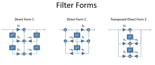
This then leads directly to the common "Direct-Form" implementations as shown in the graphic below. As MattL notes in the comments, there are additional realizations that unlike these do not derive directly from the convolution equation or generalized difference equation (for example: parallel form, frequency sampling structure, lattice and lattice-ladder, polyphase, etc) but all are ultimately mathematically equivalent to a convolution in operation.