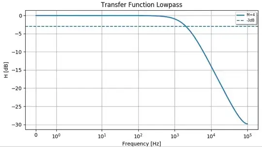
The transfer function $$H_{LPF}=\frac{b_0}{1+a_1z^{-1}}$$ becomes a multiplier-less low-pass filter if $b_0=2^{-M}$ and $a_1=2^{-M}-1$. According to this paper, the cut-off frequency is then given by $f_c=\frac{f_s}{2^M - 1}$. I tried to verify that in a python script, but I get different results. In my case, the cut-off frequency for $f_s=200kHz$ and $M=4$ is roughly at $2kHz$, whereas according to the formula it should be $13.3kHz$. Why do I get a different result?
import numpy as np
import matplotlib.pyplot as plt
from scipy import signal
from scipy.fftpack import fft
def lpf(in_signal):
    M = 4
    b = [2**(-M)]
    a = [1, 2**(-M) - 1]
return signal.lfilter(b, a, in_signal)


fs = 200e3
N_tf = 4096
u = np.concatenate(([1], np.zeros(N_tf - 1)), axis=None)
freq = np.fft.fftfreq(N_tf, 1/fs)
freq_axis = freq[0:N_tf//2]
plt.figure(figsize=(14,6), num = 'Transfer Function Lowpass')
y = lpf(u)
tf = 20*np.log10(abs(fft(y))[0:N_tf//2])
plt.plot(freq_axis, tf, linewidth = 2, label = 'M=4')
plt.axhline(-3, linestyle = 'dashed', label = '-3dB')
plt.xscale("symlog")
plt.legend(loc='upper right', shadow=True, fontsize='x-small')
plt.grid(which='both',axis='both')
plt.xlabel('Frequency [Hz]')
plt.ylabel('H [dB]')
plt.title('Transfer Function Lowpass')
plt.show()
